Kernel Ridge Regression (KRR)

Kernel Ridge Regression (KRR)#

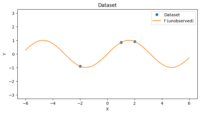
We introduce a model called Kernel Ridge Regression (KRR) that is closely related to GP regression. Like GP regression, KRR can be used to perform function approximation. We reintroduce our toy dataset from before below.

# Create dataset
f = lambda x: jnp.sin(x)
xs, ys = create_toy_dataset(f)
N = len(xs)
xs, ys

test_xs = jnp.linspace(-6, 6)
with PlotContext(title="Dataset", xlabel="X", ylabel="Y") as ax:
    plt.plot(xs, ys, marker="o", linestyle="None", label="Dataset")
    plt.plot(test_xs, f(test_xs), label="f (unobserved)")

../_images/23a6a96e390ce0f52f27e7f64deac67aaaee47b60ec430884c931c128c7e400d.png

Kernel Ridge Regression#

A Kernel Ridge Regression (KRR) is parameterized by a positive semidefinite kernel $k: \mathbb{R}^D \times \mathbb{R}^D \rightarrow \mathbb{R}$, like a GP, and weights $\alpha: \mathbb{R}^N$. We can write the prediction given by a KRR as

\[ krr(x_*; \alpha) = K_{x_* x}\alpha \]

where

$K_{x_* x} = (k(x_*, x_1) \dots k(x_*, x_N))^T$ and
$\alpha$ is a vector of $N$ weights that is learned.

def krr(k: Callable, xs: Array, alpha: Array, x_star: Array) -> Array:
    """Kernel ridge regression.
    """
    K_star_x = mk_cov(k, x_star, xs).reshape(-1)
    return K_star_x @ alpha

Learning the Weights: Loss Function#

Given a dataset $\mathcal{D} = \{(x_i, y_i) \}_{1 \leq i \leq N}$, the weights of a KRR $\alpha$ are choosen to minimize the loss function

\[\begin{align*} \mathcal{L}(\alpha; \mathcal{D}) & = (y - K_{xx}\alpha)^T\Sigma^{-1}(y - K_{xx}\alpha) + \alpha^T K_{xx} \alpha \end{align*}\]

(see Appendix: Checking Loss Minimization). The term $\alpha^T K_{xx} \alpha$ is a regularization term. The regularization term ensures that the solution is unique.

def loss(k: Callable, Sigma: Array, xs: Array, ys: Array, K_xx: Array, alpha: Array) -> float:
    """Loss function.
    """
    diff = ys.flatten() - jax.vmap(lambda x: krr(k, xs, alpha, x))(xs)
    return diff.transpose() @ jnp.linalg.inv(Sigma) @ diff + alpha.transpose() @ K_xx @ alpha

K_xx = mk_cov(k, xs, xs)
Sigma = jnp.diag(1e-2 * jnp.ones(N))

print(loss(k, Sigma, xs, ys, K_xx, jnp.array([.5, -1, .5])))
print(loss(k, Sigma, xs, ys, K_xx, jnp.array([-1, .5, .5])))
print(loss(k, Sigma, xs, ys, K_xx, jnp.array([.5, -1, -1])))

4811
8885856
2605

Learning the Weights: Solution#

The minimum can be solved in closed form and is given by

\[ \alpha = (K_{xx} + \Sigma)^{-1}y \,. \]

They can be obtained by minimizing $\mathcal{L}(\alpha; \mathcal{D})$ with respect to $\alpha$ (See Appendix: KRR). Note that this agrees with the mean of the test point prediction from a probabilistic view of a GP since the prediction

\[ krr(x_*; \alpha) = K_{*f}\alpha = K_{*f}(K_{ff} + \Sigma)^{-1}y \]

is the mean of $p(f_* | y)$.

def fit_krr(k: Callable, Sigma: Array, xs: Array, ys: Array) -> Array:
    """The same as for fitting a GP.
    """
    K_xx = mk_cov(k, xs, xs)
    alpha = jnp.linalg.inv(K_xx + Sigma) @ ys
    return K_xx, alpha

_, alpha_star = fit_krr(k, Sigma, xs, ys)
alpha_star

Array([[-0.90569925],
       [ 0.4727643 ],
       [ 0.61668825]], dtype=float32)

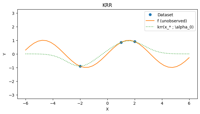
test_xs = jnp.linspace(-6, 6, 40).reshape(-1, 1)

with PlotContext(title="KRR", xlabel="X", ylabel="Y") as ax:
    # Plot dataset
    plt.plot(xs, ys, marker="o", linestyle="None", label="Dataset")
    plt.plot(test_xs, f(test_xs), label="f (unobserved)")

    # Plot KRR
    plt.plot(test_xs, [krr(k, xs, alpha_star, x) for x in test_xs], linestyle="dotted", label=r"krr(x_* ; \alpha_0)")

../_images/52a06479aa6e1017df5fb964aeb0c352777edd7aa808147a33c5b7f716a4c2b4.png

Summary#

Introduced KRR, a closely related model to GP regression.
Illustrated KRR on a toy dataset.

Appendix: KRR#

We can check that the minima of

\[ \mathcal{L}(\alpha; \mathcal{D}) = (y - K_{xx}\alpha)^T \Sigma^{-1} (y - K_{xx}\alpha) + \alpha^T K_{xx} \alpha \]

with respect to the KRR model is

\[ \alpha = (K_{xx} + \Sigma)^{-1}y \,. \]

\[\begin{align*} \operatorname{argmin}_\alpha \mathcal{L}(\alpha; \mathcal{D}) & \iff \nabla_{\alpha^T} \mathcal{L}(\alpha; \mathcal{D}) = 0 \tag{convex} \\ & \iff -K_{xx}\Sigma^{-1}y + K_{xx}\Sigma^{-1}K_{xx}\alpha + K_{MM}\alpha = 0 \tag{gradient} \\ & \iff K_{xx}\alpha + \Sigma\alpha = y \tag{multiply by $\Sigma K_{xx}^{-1}$ and rearrange} \\ & \iff \alpha = (K_{xx} + \Sigma)^{-1}y \tag{positive semi-definite} \end{align*}\]

Appendix: Checking Loss Minimization#

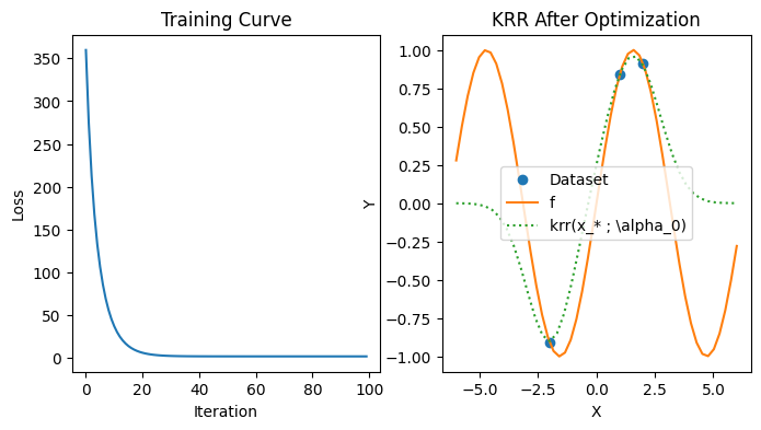
As a sanity check, we can try to minimize the loss function with gradient descent to see if we get the same answer.

def grad_desc(loss: Callable, k: Array, Sigma: Array, xs: Array, ys: Array, alpha_0, lr=0.00001, iterations=100):
    """Simple gradient descent procedure to optimize loss function.
    """
    pbar = tqdm(range(iterations))
    losses = []
    for i in pbar:
        step = lr * jax.jacrev(loss, argnums=5)(k, Sigma, xs, ys, K_xx, alpha_0)
        alpha_0 = alpha_0 - step
        l = loss(k, Sigma, xs, ys, K_xx, alpha_0)
        losses += [l]
        pbar.set_postfix(loss=l)
    return alpha_0, losses

iterations = 100
alpha_star, losses = grad_desc(loss, k, Sigma, xs, ys, jnp.ones(N), lr=0.0005, iterations=iterations)
    
plt.figure(figsize=(8, 4))
plt.subplot(1, 2, 1)
plt.plot(range(iterations), losses)
plt.title("Training Curve"); plt.xlabel("Iteration"); plt.ylabel("Loss")

plt.subplot(1, 2, 2)
plt.plot(xs, ys, marker="o", linestyle="None", label="Dataset")
plt.plot(jnp.linspace(-6, 6), f(jnp.linspace(-6, 6)), label="f")
plt.plot(test_xs, [krr(k, xs, alpha_star, x) for x in test_xs], linestyle="dotted", label=r"krr(x_* ; \alpha_0)")
plt.title("KRR After Optimization"); plt.xlabel("X"); plt.ylabel("Y"); plt.legend();

../_images/350f077a422379cbfbf1439874969819b50cce32db41388eb274421d5d6f2be0.png

# Checking that the function space and weight space solutions agree
print("alpha", jnp.linalg.inv(K_xx + Sigma) @ ys)
print("alpha_*", alpha_star)

alpha [[-0.90569925]
 [ 0.4727643 ]
 [ 0.61668825]]
alpha_* [-0.90585166  0.4838889   0.6055648 ]