import jax
from jax import random, Array
import jax.numpy as jnp
import matplotlib.pyplot as plt
from typing import *

from gp import k, mk_cov, cholesky_inv, create_toy_sparse_dataset, PlotContext

key = random.PRNGKey(42)  # Create a random key                        

Variational Gaussian Processes (VGPs)

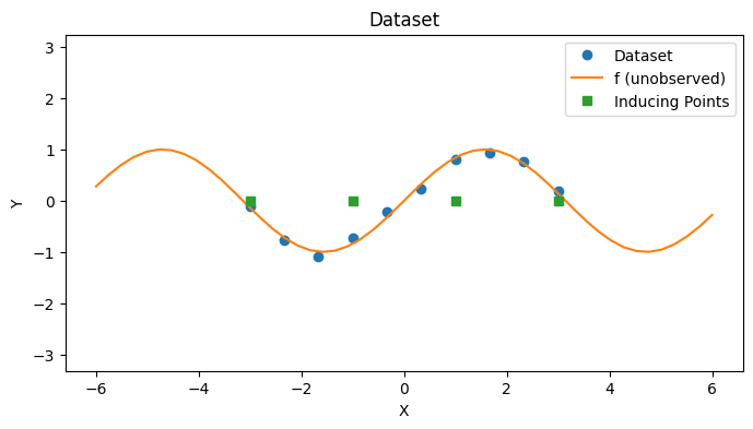
In this notebook, we explore a Variational GP (VGP) which is a kind of sparse GP aimed at solving the scaling problems of GPs by approximating the GP posterior with variational inference. As before, we’ll reintroduce a toy dataset for illustrative purposes.

# Create dataset
f = lambda x: jnp.sin(x)
xs, zs, ys, Sigma = create_toy_sparse_dataset(f, key)
N, M = len(xs), len(zs)

with PlotContext(title="Dataset", xlabel="X", ylabel="Y") as ax:
    # Plot dataset and inducing points
    plt.plot(xs, ys, marker="o", linestyle="None", label="Dataset")
    plt.plot(jnp.linspace(-6, 6), f(jnp.linspace(-6, 6)), label="f (unobserved)")
    plt.plot(zs, jnp.zeros_like(zs), marker="s", linestyle="None", label="Inducing Points")

VGP Model

In variational inference, we approximate a complex probability distribution \(p\) with a simpler distribution \(q\) from a variational family that has more tractable properties compared to \(p\). In VGP [1], we choose the distribution \(q(f, u)\) to be a approximate the posterior \(p(f, u | y)\) where \(u\) are the evaluations of a function choosen at \(M\) inducing points \(\{ z_i \}_{1 \leq i \leq M}\). That is, we will solve

\[ \operatorname{min} KL(q(f, u) || p(f, u | y)) \]

to obtain a \(q(f, u) \approx p(f, u | y)\). Posterior predictive inference can then be performed by using the posterior predictive \(q(f_* | y)\).

VGP Approximation

To construct the approximation \(q(f, u)\), we choose

\[ q(f | u) = p(f | u) \]

and solve for \(q(u)\) (See Appendix for derivation). This differs from the approach taken in SoR, which assumes that \(q(u) \sim \mathcal{N}(0, K_{uu})\) and approximates \(p(f | u) \approx q_{SoR}(f | u)\). Titsias shows that

\[\begin{align*} q(u) & = \mathcal{N}(u \,|\, K_{zz}C^{-1}K_{zx}\Sigma^{-1} y, K_{zz}C^{-1}K_{zz}) \end{align*}\]

where \(C = K_{zz} + K_{zx}\Sigma^{-1} K_{xz}\).

# Compute kernel
K_zz = mk_cov(k, zs, zs)
K_zx = mk_cov(k, zs, xs)
K_xz = K_zx.transpose()

# Compute mean and covariance
Sigma_inv = cholesky_inv(Sigma)
C = K_zz + K_zx @ Sigma_inv @ K_xz
C_inv = cholesky_inv(C)
m = (K_zz @ C_inv @ K_zx @ Sigma_inv @ ys).reshape(-1)
cov = K_zz @ C_inv @ K_zz

# Sample q(u)
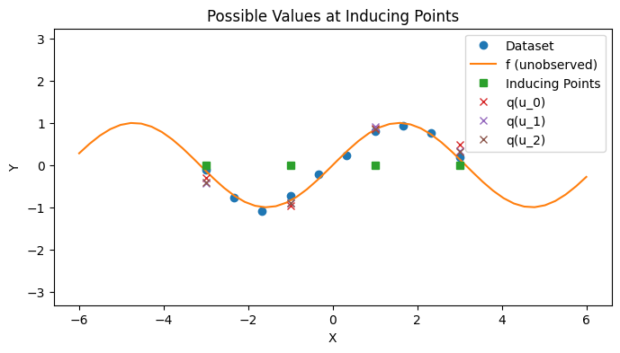
us = random.multivariate_normal(key, mean=m, cov=cov, shape=(3,)).transpose()

with PlotContext(title="Possible Values at Inducing Points", xlabel="X", ylabel="Y") as ax:
    # Plot dataset and inducing points
    plt.plot(xs, ys, marker="o", linestyle="None", label="Dataset")
    plt.plot(jnp.linspace(-6, 6), f(jnp.linspace(-6, 6)), label="f (unobserved)")

    # Plot q(u)
    plt.plot(zs, jnp.zeros_like(zs), marker="s", linestyle="None", label="Inducing Points")
    for i in range(3):
        plt.plot(zs, us[:, i], marker="x", linestyle="None", label=f"q(u_{i})")

Fitting a VGP

The posterior predictive of a VGP (see Titsias [2], eq 6 and also the Appendix) is

\[\begin{align*} q(f_* | y) & = \mathcal{N}(K_{*z}C^{-1}K_{zx}\Sigma^{-1}y, K_{* *} - K_{*z}(K_{zz}^{-1} - C^{-1})K_{z*}) \,. \end{align*}\]

As a reminder, \(C = K_{zz} + K_{zx}\Sigma^{-1} K_{xz}\).

def fit_vgp(k: Callable, Sigma: Array, xs: Array, ys: Array, zs: Array):
    # Compute covariances
    K_zz = mk_cov(k, zs, zs)
    K_xz = mk_cov(k, xs, zs)
    K_zx = K_xz.transpose()
    K_zz_inv = cholesky_inv(K_zz)
    
    # Perform approximations
    Sigma_inv = cholesky_inv(Sigma)
    C = K_zz + K_zx @ Sigma_inv @ K_xz
    C_inv = cholesky_inv(C)
    
    alpha = C_inv @ K_zx @ Sigma_inv @ ys
    cov = K_zz_inv - C_inv
    
    return alpha, cov, K_zz, K_zz_inv

def vgp_post_pred_mean(k: Callable, zs: Array, alpha: Array, x_star: Array) -> Array:
    """Posterior predictive mean.
    """
    K_star_z = mk_cov(k, x_star, zs).reshape(-1)
    return K_star_z @ alpha


def vgp_post_pred_cov(k: Callable, zs: Array, cov: Array, x_star: Array) -> Array:
    """Posterior predictive covariance.
    """
    K_star_star = mk_cov(k, x_star, x_star)
    K_star_z = mk_cov(k, x_star, zs)
    return K_star_star - K_star_z @ cov @ K_star_z.transpose()

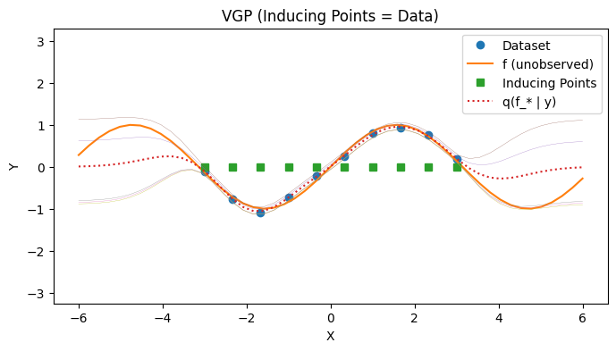
Visualizing the Posterior Predictive 1: No Inducing Points

# Fit
zs_all_xs = xs
alpha_all_xs, cov_all_xs, K_zz_all_xs, K_zz_inv_all_xs = fit_vgp(k, Sigma, xs, ys, zs_all_xs)

# Predict
test_xs = jnp.linspace(-6, 6).reshape(-1, 1)
post_ys = [vgp_post_pred_mean(k, zs_all_xs, alpha_all_xs, x) for x in test_xs]
post_mean = jax.vmap(lambda x_star: vgp_post_pred_mean(k, zs_all_xs, alpha_all_xs, x_star))(test_xs)
post_cov = jax.vmap(lambda x_star: vgp_post_pred_cov(k, zs_all_xs, cov_all_xs, x_star), out_axes=0)(test_xs)
post_cov_ys = [random.normal(key, shape=(5,)) * jnp.sqrt(post_cov[i][0][0]) + post_mean[i] for i in range(len(test_xs))]

with PlotContext(title="VGP (Inducing Points = Data)", xlabel="X", ylabel="Y") as ax:
    # Plot dataset and inducing points
    plt.plot(xs[:,0], ys, marker='o', linestyle='none', label="Dataset")
    plt.plot(jnp.linspace(-6, 6), f(jnp.linspace(-6, 6)), label="f (unobserved)")
    plt.plot(zs_all_xs, jnp.zeros_like(zs_all_xs), marker="s", linestyle="None", label="Inducing Points")

    # Plot p(f(*) | y)
    plt.plot(test_xs, post_ys, label="q(f_* | y)", linestyle="dotted")
    plt.plot(test_xs, post_cov_ys, linewidth=0.2)

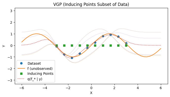
Visualizing the Posterior Predictive 2: Subset

# Fit
zs_p = jnp.array([xs[0], xs[1], xs[-3]])
alpha_p, cov_p, K_zz_p, K_zz_inv_p = fit_vgp(k, Sigma, xs, ys, zs_p)

# Predict
test_xs = jnp.linspace(-6, 6).reshape(-1, 1)
post_ys = [vgp_post_pred_mean(k, zs_p, alpha_p, x) for x in test_xs]
post_mean = jax.vmap(lambda x_star: vgp_post_pred_mean(k, zs_p, alpha_p, x_star))(test_xs)
post_cov = jax.vmap(lambda x_star: vgp_post_pred_cov(k, zs_p, cov_p, x_star), out_axes=0)(test_xs)
post_cov_ys = [random.normal(key, shape=(5,)) * jnp.sqrt(post_cov[i][0][0]) + post_mean[i] for i in range(len(test_xs))]

# Plot
with PlotContext(title="VGP (Inducing Points Subset of Data)", xlabel="X", ylabel="Y") as ax:
    # Plot dataset and inducing points
    plt.plot(xs[:,0], ys, marker='o', linestyle='none', label="Dataset")
    plt.plot(jnp.linspace(-6, 6), f(jnp.linspace(-6, 6)), label="f (unobserved)")
    plt.plot(zs_all_xs, jnp.zeros_like(zs_all_xs), marker="s", linestyle="None", label="Inducing Points")

    # Plot p(f(*) | y)
    plt.plot(test_xs, post_ys, label="q(f_* | y)", linestyle="dotted")
    plt.plot(test_xs, post_cov_ys, linewidth=0.2)

Summary

1. We have seen how variational inference can be applied to make GP inference tractable.

2. We have illustrated VGP on a toy dataset.

References

1. Variational Model Selection for Sparse Gaussian Process Regression

2. Variational Learning of Inducing Variables in Sparse Gaussian Processes

Appendix

Appendix: VGP Derivation

We want to solve

\[ \operatorname{min} KL(q(f, u) || p(f, u | y)) \]

where

\[ q(f, u) = p(f | u) q(u) \,. \]

Titsias shows that

\[\begin{align*} q(u) & = \mathcal{N}(u \,|\, K_{zz}C^{-1}K_{zx}\Sigma^{-1} y, K_{zz}C^{-1}K_{zz}) \end{align*}\]

where \(C = K_{zz} + K_{zx}\Sigma^{-1} K_{xz}\).

Generative Process

As a reminder, the generative process for a GP with inducing points is

\[\begin{align*} u(z) & \sim \mathcal{N}(0, K_{zz}) \\ f(x) \,|\, u(z) & \sim \mathcal{N}(K_{xz}K_{zz}^{-1}u(z), K_{xx} - Q_{xx}) \\ \epsilon & \sim \mathcal{N}(0, \Sigma) \\ y & = f(x) + \epsilon \end{align*}\]

where \(\Sigma = \beta^2I\) and \(Q_{xx} = K_{xz}K_{zz}^{-1}K_{zx}\). We will abbreviate \(u(z) = u\) and \(f(x) = f\).

Note that

\[\begin{split} p(f, u) = \mathcal{N} \left(f, u | 0, \begin{pmatrix} K_{xx} & K_{xz} \\ K_{zx} & K_{zz} \end{pmatrix} \right) \,. \end{split}\]

VGP Derivation: ELBO

Titsias shows in Appendix A [1] that

(1)\[\begin{align} \text{ELBO}(q(f, u)) & = \int q(f, u) \log \frac{p(y, f, u)}{q(f, u)} df du \tag{defn ELBO} \\ & = \int p(f \,|\, u) q(u) \log \frac{p(y \,|\, f) p(f \,|\, u) p(u)}{p(f \,|\, u) q(u)} df du \tag{defn $p$ and $q$} \\ & = \int p(f \,|\, u) q(u) \log \frac{p(y \,|\, f) p(u)}{q(u)} df du \tag{cancel} \\ & = \int \left[ \int \left( \log p(y \,|\, f) + \log \frac{p(u)}{q(u)} \right) p(f \,|\, u) df \right] q(u) du \tag{rearrange} \\ & = \int \left[ \int \log p(y \,|\, f) \cdot p(f \,|\, u) df + \log \frac{p(u)}{q(u)} \right] q(u) du \tag{linearity and integrate} \,. \end{align}\]

VGP Derivation: ELBO Inner Integral

We solve for the inner integral. Titsias further shows in Appendix A [1] that

\[\begin{align*} & \phantom{=} \int \log p(y \,|\, f) \cdot p(f \,|\, u) df \notag \\ & = \int \log \left[ (2\pi)^{-N/2} \beta^{-N} \exp \left( -\frac{1}{2} (y - f)^T\Sigma^{-1}(y - f) \right) \right] p(f \,|\, u) df \tag{Gaussian pdf} \\ & = \int \left[ -\frac{N}{2} \log 2\pi\beta^2 + \left( -\frac{1}{2} (y - f)^T\Sigma^{-1}(y - f) \right) \right] p(f \,|\, u) df \tag{log} \\ & = \int \left[ -\frac{N}{2} \log 2\pi\beta^2 - \frac{1}{2\beta^2}Tr(yy^T - 2y f^T + ff^T) \right] p(f \,|\, u) df \tag{trace rearrange} \\ & = -\frac{N}{2} \log 2\pi\beta^2 - \frac{1}{2\beta^2} \int Tr(yy^T - 2y f^T + ff^T) p(f \,|\, u) df \tag{linearity and integrate} \\ & = -\frac{N}{2} \log 2\pi\beta^2 - \frac{1}{2\beta^2} \int (Tr(yy^T) - Tr(2y f^T) + Tr(ff^T)) p(f \,|\, u) df \tag{linearity trace} \\ & = -\frac{N}{2} \log 2\pi\beta^2 - \frac{1}{2\beta^2} \left((Tr(yy^T) + \int - Tr(2y f^T) + Tr(ff^T)) p(f \,|\, u) df \right) \tag{indep} \\ & = -\frac{N}{2} \log 2\pi\beta^2 - \frac{1}{2\beta^2} \left((Tr(yy^T) - Tr(2y \alpha^T) + \int Tr(ff^T)) p(f \,|\, u) df \right) \tag{mean} \\ & = -\frac{N}{2} \log 2\pi\beta^2 - \frac{1}{2\beta^2} \left((Tr(yy^T) - Tr(2y \alpha^T) + Tr(\alpha\alpha^T + B) \right) \tag{second moment} \\ & = -\frac{N}{2}\log 2\pi\beta^2 - \frac{1}{2\beta^2}Tr(yy^T - 2y\alpha^T + \alpha\alpha^T) - \frac{1}{2\beta^2}Tr(B) \tag{linearity trace} \\ & = -\frac{N}{2}\log 2\pi\beta^2 - \frac{1}{2\beta^2}(y - \alpha)^T \Sigma^{-1}(y - \alpha)- \frac{1}{2\beta^2}Tr(B) \tag{algebra} \\ & = \log \mathcal{N}(y \,|\, \alpha, \Sigma) - \frac{1}{2\beta^2}Tr(B) \tag{Gaussian pdf} \end{align*}\]

where \(\alpha = K_{xz}K_{zz}^{-1}u\) is mean of \(p(f \,|\, u)\) and \(B = K_{xx} - Q_{xx}\) is covariance of \(p(f \,|\, u)\).

VGP Derivation: Continue ELBO Simplification

We can now continue to simplify the ELBO.

\[\begin{align*} \text{ELBO}(q(f, u)) & = \int \left[ \int \log p(y \,|\, f) \cdot p(f \,|\, u) df + \log \frac{p(u)}{q(u)} \right] q(u) du \tag{defn} \\ & = \int \left[ \log \mathcal{N}(y \,|\, \alpha, \Sigma) - \frac{1}{2\beta^2}Tr(B) + \log \frac{p(u)}{q(u)} \right] q(u) du \tag{previous} \\ & = \int \left[ \log \mathcal{N}(y \,|\, \alpha, \Sigma) + \log \frac{p(u)}{q(u)} \right] q(u) du - \frac{1}{2\beta^2}Tr(B) \tag{linearity and integrate} \\ & = \int \left[ \log \frac{\mathcal{N}(y \,|\, \alpha, \Sigma) p(u)}{q(u)} \right] q(u) du - \frac{1}{2\beta^2}Tr(B) \tag{log, Eq *} \\ & \leq \log \int \left[\frac{\mathcal{N}(y \,|\, \alpha, \Sigma) p(u)}{q(u)} \right] q(u) du - \frac{1}{2\beta^2}Tr(B) \tag{Jensen's} \\ & \leq \log \int \mathcal{N}(y \,|\, \alpha, \Sigma) p(u) du - \frac{1}{2\beta^2}Tr(B) \tag{simpl} \\ & = \log \int \mathcal{N}\left( \begin{pmatrix} y \\ u \end{pmatrix} \,|\, \begin{pmatrix} 0 \\ K_{xz}K_{zz}^{-1}u \end{pmatrix}, \begin{pmatrix} K_{zz} & K_{zx} \\ K_{xz} & \Sigma \end{pmatrix}\right) du - \frac{1}{2\beta^2}Tr(B) \tag{joint/cond} \\ & = \log \mathcal{N}(y \,|\, 0, \Sigma + K_{xz}K_{zz}^{-1}K_{zx}) - \frac{1}{2\beta^2}Tr(B) \tag{marg} \end{align*}\]

VGP Derivation: Solving ELBO for q(u) step 1

We now need to find the optimal \(q(u)\). We can see that \(q(u) \propto \mathcal{N}(y \,|\, \alpha, \Sigma) p(u)\) by differentiating the ELBO at Eq * w.r.t. \(q(u)\) and setting it to \(0\).

\[\begin{align*} q(u) & \propto \mathcal{N}(y \,|\, \alpha, \Sigma) p(u) \tag{*} \\ & = c_1 \exp\left[ -\frac{1}{2}(y - \alpha)^T\Sigma^{-1} (y - \alpha) \right] c_2 \exp\left[ -\frac{1}{2}u^T K_{zz}^{-1}u \right] \tag{pdf} \\ & = c_1 c_2 \exp\left[ -\frac{1}{2}(y - \alpha)^T\Sigma^{-1} (y - \alpha) -\frac{1}{2}u^T K_{zz}^{-1}u \right] \tag{simpl} \\ & = c_1 c_2 \exp\left[ -\frac{1}{2}\left( y^T\Sigma^{-1} y - 2y^T \Sigma^{-1} \alpha + \alpha^T \Sigma^{-1} \alpha + u^T K_{zz}^{-1}u \right) \right] \tag{simpl} \\ & = c_1 c_2 c_3 \exp\left[ -\frac{1}{2}\left(-2y^T \Sigma^{-1} \alpha + \alpha^T \Sigma^{-1} \alpha + u^T K_{zz}^{-1}u \right) \right] \tag{simpl} \\ & = c \exp\left[ -\frac{1}{2}\left(-2y^T \Sigma^{-1} (K_{xz}K_{zz}^{-1}u) + u^T K_{zz}^{-1} K_{zx} \Sigma^{-1} K_{xz}K_{zz}^{-1}u + u^T K_{zz}^{-1}u \right) \right] \tag{defn $\alpha$} \\ & = c \exp\left[ -\frac{1}{2}\left(u^T (K_{zz}^{-1} + K_{zz}^{-1} K_{zx} \Sigma^{-1} K_{xz}K_{zz}^{-1})u - 2y^T \Sigma^{-1} K_{xz}K_{zz}^{-1}u \right) \right] \tag{rearrange} \end{align*}\]

VGP Derivation: Solving ELBO for q(u) step 2

We can complete the square using

\[\begin{align*} x^TMx - 2b^Tx = (x - M^{-1}b)^TM(x - M^{-1}b) - b^Tb \end{align*}\]

to obtain

\[\begin{align*} q(u) = \mathcal{N}(u \,|\, D^{-1}K_{zz}^{-1}K_{zx}\Sigma^{-1} y, D^{-1}) \end{align*}\]

where

\[\begin{align*} D = K_{zz}^{-1}K_{zx}\Sigma^{-1} K_{xz}K_{zz}^{-1} + K_{zz}^{-1} \,. \end{align*}\]

Titsias further simplies this to

\[\begin{align*} q(u) & = \mathcal{N}(u \,|\, K_{zz}C^{-1}K_{zx}\Sigma^{-1} y, K_{zz}C^{-1}K_{zz}) \end{align*}\]

where \(C = K_{zz} + K_{zx}\Sigma^{-1} K_{xz}\) as required.

Appendix: Posterior Predictive

Variational Family

Note that

\[\begin{split} q(f, u) = \mathcal{N} \left( \begin{pmatrix} f \\ u \\ \end{pmatrix} | \begin{pmatrix} K_{xz}K_{zz}^{-1}m \\ m \\ \end{pmatrix}, \begin{pmatrix} K_{xx} - K_{xz}K_{zz}^{-1}(K_{zz} - A)K_{zz}^{-1}K_{zx} & K_{xz}K_{zz}^{-1}A \\ AK_{zz}^{-1}K_{zx} & A \\ \end{pmatrix} \right) \end{split}\]

where

1. \(m = K_{zz} C^{-1} K_{zx}\Sigma^{-1}y\),

2. \(A = K_{zz} C^{-1} K_{zz}\), and

3. \(C = (K_{zz} + K_{zx}\Sigma^{-1}K_{xz})\).

Computing Posterior Predictive

\[\begin{align*} q(f(*) \,|\, y) & = \int p(f(*) \,|\, f, u) q(f, u) df du \tag{marg} \\ & = \int p(f(*) \,|\, f, u) p(f \,|\, u) q(u) df du \tag{factor} \\ & = \int p(f(*), f \,|\, u) q(u) df du \tag{factor} \\ & = \int q(*, u) du \tag{defn} \\ & = \mathcal{N}(K_{*z}K_{zz}^{-1}m, K_{* *} - K_{*z}K_{zz}^{-1}(K_{zz} - A)K_{zz}^{-1}K_{z*}) \tag{marg} \\ & = \mathcal{N}(K_{*z}K_{zz}^{-1}K_{zz} C^{-1} K_{zx}\Sigma^{-1}y, K_{* *} - K_{*z}K_{zz}^{-1}(K_{zz} - A)K_{zz}^{-1}K_{z*}) \tag{subst m} \\ & = \mathcal{N}(K_{*z} C^{-1} K_{zx}\Sigma^{-1}y, K_{* *} - K_{*z}K_{zz}^{-1}(K_{zz} - A)K_{zz}^{-1}K_{z*}) \tag{simplify} \\ & = \mathcal{N}(K_{*z} C^{-1} K_{zx}\Sigma^{-1}y, K_{* *} - K_{*z}K_{zz}^{-1}K_{z*} + K_{*z}K_{zz}^{-1}AK_{zz}^{-1}K_{z*}) \tag{distribute} \\ & = \mathcal{N}(K_{*z} C^{-1} K_{zx}\Sigma^{-1}y, K_{* *} - K_{*z}K_{zz}^{-1}K_{z*} + K_{*z}C^{-1}K_{z*}) \tag{subst A} \\ & = \mathcal{N}(K_{*z} C^{-1} K_{zx}\Sigma^{-1}y, K_{* *} - K_{*z}(K_{zz}^{-1} - C^{-1})K_{z*}) \tag{rearrange} \\ \end{align*}\]