import numpy as np
from qutip import sigmaz, mesolve, Bloch, Qobj

from util import pretty
Adiabatic Quantum Computing#
We introduce adiabatic quantum computing (AQC) in this notebook. AQC applies perturbations to the Hamiltonian of a quantum system to transform the quantum state by the adiabatic theorem. Thus, AQC is a form of analog QC which relies on a different aspect of quantum mechanics to perform QC.
Review: Hamiltonian#
As a reminder, a Hamiltonian for a quantum system with \(n\) qubits of information can be encoded as a \(2^N \times 2^N\) Hermitian matrix where \(N = 2^N\) encoding the total energy of a quantum system.
# Example Hamiltonian
H = Qobj(np.array([
    [0, -1j],
    [1j, 0]
]), dims=[[2], [2]])
pretty(H.full())
Spectral Decomposition#
By the Spectral Decomposition, every Hermitian matrix can be diagonalized:
where \(U\) is an orthonormal matrix of eigenvectors and \(\Lambda\) is a diagonal matrix containing the eigenvalues. Recall that \(U^{-1} = U^*\) when \(U\) is orthonormal.
# Eigenvector/eigenvalue decompostion
eigenvalues, eigenvectors = np.linalg.eigh(H.full())
print("Eigenvalues", eigenvalues)
print("Eigenvectors")
pretty(eigenvectors)
Eigenvalues [-1.  1.]
Eigenvectors
H_reconstructed = eigenvectors @ np.diag(eigenvalues) @ np.conjugate(eigenvectors).T
np.allclose(H.full(), H_reconstructed)
True
Ground State and Energy#
The eigenvalues of a Hamiltonian can be interpreted as energies. Recall that a Hermitian matrix has real eigenvalues so that energies are real numbers. The smallest eigenvalue is called the ground energy.
The eigenvector associated with the smallest eigenvalue of a Hamiltonian can be interpreted as a ground state.
print("All real eigenvalues", [np.allclose(ev.imag, 0j) for ev in eigenvalues])
print("Ground energy", eigenvalues[0])
print("Ground state")
pretty(eigenvectors[0])
All real eigenvalues [True, True]
Ground energy -1.0
Ground state
print("Ground energy", H.groundstate()[0])
print("Ground state")
pretty(H.groundstate()[1])
Ground energy -1.0
Ground state
Adiabatic Evolution#
AQC relies on the adiabatic theorem to perform computation. Given a time-dependent Hamiltonian \(H_t\) on a time interval \([0, T]\) that meets certain conditions, the quantum state of a quantum system under adiabatic evolution will transition from the ground state of \(H_0\) to the ground state of \(H_T\). That is,
if \(H_t\) satisfies certain conditions given by the adiabatic theorem. Thus, we require several ingredients to perform AQC:
a time-varying Hamiltonian \(H_t\) that meets the conditions of the adiabatic theorem and
a method to compute the time \(T\) that also meets the conditions of the adiabatic theorem.
We’ll discuss this in turn.
Time-Varying Hamiltonian#
A commonly-used time-dependent Hamiltonian for AQC is
which linearly interpolates between \(H_0\) and \(H_T\). This meets one of the conditions of an adiabatic theorem which requires that \(H_t\) be “smooth” in \(t\). We’ll given an example now that puts \(\ket{1}\) in superposition
H_0 = sigmaz()
pretty(H_0.full())
# Initial state is |1>
global_phase = np.exp(-1j * np.pi)
pretty(global_phase * H_0.groundstate()[-1])
# Final state is |->
H_T = Qobj(np.array([
    [0, 0.5],
    [0.5, 0]
]), dims=[[2], [2]])
pretty(global_phase * H_T.groundstate()[-1])
def linear_interpolation(H_0, H_T, T):
    def s(t):
        return t / T
    H_t = [[H_0, lambda t: 1 - s(t)], [H_T, s]]
    return H_t

linear_interpolation(H_0, H_T, 10)
[[Quantum object: dims=[[2], [2]], shape=(2, 2), type='oper', dtype=CSR, isherm=True
  Qobj data =
  [[ 1.  0.]
   [ 0. -1.]],
  <function __main__.linear_interpolation.<locals>.<lambda>(t)>],
 [Quantum object: dims=[[2], [2]], shape=(2, 2), type='oper', dtype=Dense, isherm=True
  Qobj data =
  [[0.  0.5]
   [0.5 0. ]],
  <function __main__.linear_interpolation.<locals>.s(t)>]]
Computing the Evolution Time#
The time \(T\) is inversely related to the spectral gap which is the minimum difference between the lowest and second-lowest eigenvalues of the Hamiltonian of \(H_t\). Thus, the larger the spectral gap, the shorter the time \(T\), and vice versa. Thus the spectral gap governs how “slowly” we must vary the Hamiltonian in order to perform adiabatic evolution. In general, we must analyze \(H_t\) on a case-by-case basis to determine the best (i.e., shortest) \(T\).
# Let's be conservative
T = 10
Putting it Together#
Define an adiabatic quantum program as a tuple
where \(H_t\) is a time-dependent Hamiltonian defined for \(t \in [0, T]\) and such that \(H_t\) has a unique ground state \(\ket{\psi(t)}\) for all \(0 \leq t \leq T\) where \(T\) is the length of simulation. Then
in time \(T\).
# Adiabatic program
T = 5*np.pi
H_t = linear_interpolation(H_0, H_T, T)
psi_0 = global_phase * H_0.groundstate()[-1]  # Initial state
psi_T = global_phase * H_T.groundstate()[-1]  # Final state
# Simulation
times = np.linspace(0, T, 500)
result = mesolve(H_t, psi_0, times, [], [])
psi_T_sim = global_phase * result.states[-1]
pretty(psi_T_sim)
We can plot the answer on a Bloch sphere.
b = Bloch()
b.add_states(psi_T_sim)
b.add_annotation(psi_T_sim, "S", color='b')  # S for simulated
b.add_states(psi_T)
b.add_annotation(psi_T, "R", color='r')      # R for real
b.show()
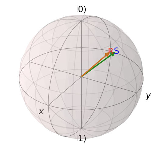
We can also check the overlap.
overlap = abs(psi_T_sim.overlap(psi_T))**2
print(f"Overlap with ground state of final Hamiltonian: {overlap:.4f}")
Overlap with ground state of final Hamiltonian: 0.9963
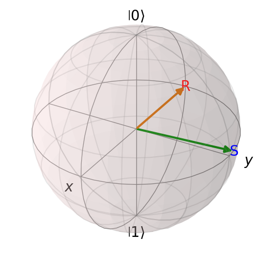
Shorter Time#
If we try to run for too short of a time, we risk perturbing the Hamiltonian at too fast a rate. Therefore, our computation will not produce the desired effect.
# Adiabatic program
T = np.pi
H_t = linear_interpolation(H_0, H_T, T)

# Simulation
times = np.linspace(0, T, 500)
result = mesolve(H_t, psi_0, times, [], [])
psi_T_sim = result.states[-1]

overlap = abs(psi_T_sim.overlap(psi_T))**2
print(f"Overlap with ground state of final Hamiltonian: {overlap:.4f}")

b = Bloch()
b.add_states(psi_T_sim)
b.add_annotation(psi_T_sim, "S", color='b')  # S for simulated
b.add_states(psi_T)
b.add_annotation(psi_T, "R", color='r')      # R for real
b.show()
Overlap with ground state of final Hamiltonian: 0.7696
Summary#
We have reviewed the ground state and ground energy of a Hamiltonian.
We have seen how AQC performs computation by transitioning from the ground state of an initial Hamiltonian to the ground state of a final hamiltonian by perturbing a Hamiltonian over time.
The time that we run an adiabatic computation affects the fidelty of our result.
References#
[1] On the Adiabatic Theorem of Quantum Mechanics
[2] Adiabatic Quantum Computation is Equivalent to Standard Quantum Computation
[3] The quantum adiabatic optimization algorithm and local minima
[4] Lecture 18: The quantum adiabatic theorem by Prof. Andrew Childs
Appendix: Adiabatic Theorem#
Preliminaries#
Define \(\Delta(H)\) to be the spectral gap of a Hamiltonian H, to be the difference between the lowest eigenvalue of H and its second lowest eigenvalue.
def spectral_gap(H: np.ndarray) -> float:
    eigvals, _ = np.linalg.eigh(H.full())
    idxs = np.argsort(eigvals)
    for idx in idxs[1:]:
        if eigvals[idx] > eigvals[0]:
            return eigvals[idx] - eigvals[0]
    return 0

spectral_gap(H_0), spectral_gap(H_T)
(2.0, 1.0)
Define the spectral norm
print("||H_0||", np.linalg.norm(H_0.full(), ord=2))
print("||H_T||", np.linalg.norm(H_T.full(), ord=2))
||H_0|| 1.0
||H_T|| 0.5
Adiabatic Theorem (Theorem 2.1 [2] and [3])#
Let \(H_{\text{init}}\) and \(H_{\text{final}}\) be two Hamiltonians acting on a quantum system. Define
and assume that \(H(s)\) has a unique ground state for all \(s\).
Then for any fixed \(\delta > 0\), if
then the final state of an adiabatic evolution according to \(H\) for time \(T\) (with an appropriate setting of global phase) is \(\epsilon\)-close in \(\ell_2\)-norm to the ground state of \(H_{\text{final}}\).