from bloqade import start
from qutip import basis, mesolve, Qobj, QobjEvo
import matplotlib.pyplot as plt
import numpy as np

from util import pretty, mk_H_Rydberg, histogram_final_state, plot_histogram, invert_keys
Adiabatic Quantum Computing with Neutral Atoms#
In this notebook, we will introduce adiabatic quantum computing (AQC) with neutral atoms.
Review: Adiabatic Quantum Computing#
Recall that an adiabatic quantum program is a tuple
where \(H_t\) is a time-dependent Hamiltonian defined for \(t \in [0, T]\) and such that \(H_t\) has a unique ground state \(\ket{\psi(t)}\) for all \(0 \leq t \leq T\) where \(T\) is the length of simulation.
An adiabatic evolution then performs the computation
in time \(T\).
Example: \(\ket{0} \rightarrow \ket{1}\)#
We will now set up a computation that flips a qubit from \(\ket{0}\) to \(\ket{1}\). As a reminder, the Rydberg Hamiltonian on a single qubit (i.e., Rydberg atom) is given as
where
\(\Omega(t)\) is a Rabi frequency,
\(\phi(t)\) is the Rabi phase, and
\(\Delta(t)\) is the detuning of the driving laser.
Initial Hamiltonian#
We need to construct a Rydberg Hamiltonian whose ground state is \(\ket{0}\). One such Hamiltonian is given below where we set the detuning to a negative number.
Omega_init = 0
phi = 0
Delta_init = -30
register = start.add_position([(0, 0)])  # (um)
H_init = mk_H_Rydberg(1, Omega_init, phi, Delta_init, register)
pretty(H_init)
eigvals, eigs = np.linalg.eigh(H_init)
idxs = np.argsort(eigvals)
assert eigvals[idxs[0]] < np.max(eigvals[idxs[1:]])
print(eigvals[idxs])
pretty(eigs[:, idxs[0]])
[ 0. 30.]
Final Hamiltonian#
Next, we construct a Rydberg Hamiltonian whose ground state is \(\ket{1}\). One such Hamiltonian is given below where we set the detuning to a positive number.
Omega_final = 0
Delta_final = 30
H_final = mk_H_Rydberg(1, Omega_final, phi, Delta_final, register)
pretty(H_final)
eigvals, eigs = np.linalg.eigh(H_final)
idxs = np.argsort(eigvals)
assert eigvals[idxs[0]] < np.max(eigvals[idxs[1:]])
print(eigvals[idxs])
pretty(eigs[:, idxs[0]])
[-30. 0.]
Bloqade Program#
We can now construct a Bloqade program to perform this adiabatic computation. One issues is that we require a non-zero \(\Omega\) at some point during the computation. Otherwise, our qubits will not oscillate between \(\ket{0}\) and \(\ket{1}\). To accomplish this we can ramp up \(\Omega\) from \(0\) to \(15\) and back down to \(0\) to match our intial and final Hamiltonian above. If we perform these transitions slowly enough, the adiabatic theorem will apply and we will successfully perform our computation.
T = np.pi*4
register = start.add_position([(0, 0)])  # (um)
program = (
    register
    .rydberg.rabi.amplitude.uniform.piecewise_linear(
        durations=[0.2, T - 0.4, 0.2],
        values=[0, 15, 15, 0]
    )
    .rydberg.rabi.phase.uniform.piecewise_constant(
        durations=[T],
        values=[0]
    )
    .rydberg.detuning.uniform.piecewise_linear(
        durations=[T],
        values=[-30, 30]
    )
)
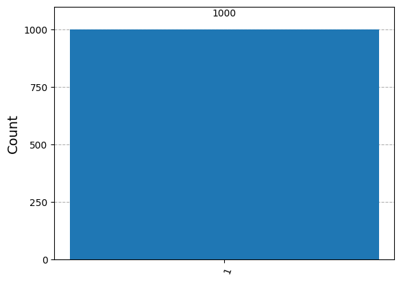
results = program.bloqade.python().run(1000)
report = results.report()
plot_histogram(invert_keys(report.counts()))
QuTip Solving#
We can also manually implement this Rydberg Hamiltonian using the more generic qutip library as a sanity check.
T = np.pi*4
phi = 0
times = np.linspace(0, T, 500)
def Omega(t):
if t < 0.2:
return 15/.2*t
elif t < T - 0.2:
return 15
else:
t = T - t
return 15/.2*t
def Delta(t):
return Delta_init + (Delta_final - Delta_init)/T*t
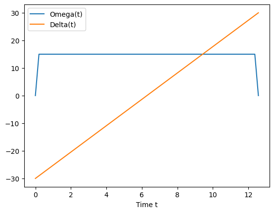
plt.plot(times, [Omega(t) for t in times], label="Omega(t)")
plt.plot(times, [Delta(t) for t in times], label="Delta(t)")
plt.legend()
plt.xlabel("Time t")
Text(0.5, 0, 'Time t')
# Construct the time-dependent Hamiltonian
H_list = [Qobj(mk_H_Rydberg(1, Omega(t), phi, Delta(t), register), dims=[[2], [2]]) for t in times]
H = QobjEvo(H_list, tlist=times)
result = mesolve(H, basis(2, 0), times, [], [])
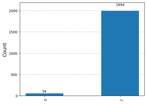
pretty(result.final_state)
plot_histogram(histogram_final_state(result.final_state))
Summary#
We saw a simple example of performing an adiabatic computation with neutral atoms.