from qiskit import QuantumCircuit, QuantumRegister, ClassicalRegister

from pulser import Pulse, Sequence, Register
from pulser.devices import DigitalAnalogDevice
from pulser.waveforms import BlackmanWaveform
from pulser_patch.simulation import QutipEmulator
import matplotlib.pyplot as plt

import numpy as np
from util import plot_histogram, simulate

Pulse-Level Quantum Computing with Neutral Atoms

In this notebook, we introduce neutral atom quantum computing with pulse sequences. Pulse sequences enable us to control a quantum computer in both digital and analog modes.

Programming with Pulse Sequences

As a reminder, a program for a neutral atom computer consists of

1. a register defining the locations of the qubits and

2. waveforms for the Rabi frequency \(\Omega_j\), Rabi phase \(\phi_j\), and detuning \(\Delta\).

These are inputs to to the Rydberg Hamiltonian, reproduced below

\[ \frac{H(t)}{\hbar} = \frac{\Omega(t)}{2} \sum_{j=1}^n (e^{i\phi_j(t)} |g_j\rangle\langle r_j| + e^{-i\phi_j(t)} |r_j\rangle\langle g_j|) -\Delta(t) \sum_{j=1}^n \hat{n}_j + \sum_{j < k} V_{jk} \hat{n}_j\hat{n}_k \,. \]

Example: Bell State

Following [1], we’ll use pulse sequences to construct a Bell state. First, we’ll review a gate-based program that constructs the Bell-state before mimicing it with a pulse sequence.

Gate-Based Program

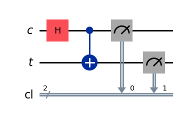
The standard gate-based program uses a Hadamard gate followed by a CX gate.

qc = QuantumCircuit(QuantumRegister(1, "c"), QuantumRegister(1, "t"), ClassicalRegister(2, "cl"))
qc.h(0)
qc.cx(0, 1)
qc.measure(range(2), range(2))
qc.draw(output="mpl")

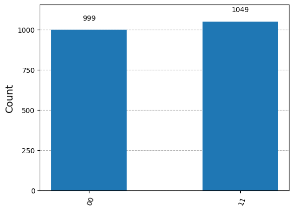
After running this circuit, we obtain the Bell state

\[ \frac{1}{\sqrt{2}}(\ket{00} + \ket{11}) \,. \]

counts = simulate(qc)
plot_histogram(counts)

Equivalent Gate-Based Program

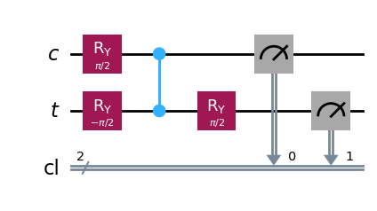
On a neutral atom computer, it will be easier to apply \(RY(\theta)\) (i.e., rotation around \(y\)-axis on the Bloch sphere) and the \(CZ\) gate (i.e., controlled \(RZ\) gate). We can rewrite the program above equivalently using only \(RY(\theta)\) and \(CZ\) gates.

qc_equiv = QuantumCircuit(QuantumRegister(1, "c"), QuantumRegister(1, "t"), ClassicalRegister(2, "cl"))
qc_equiv.ry(np.pi/2, 0)
qc_equiv.ry(-np.pi/2, 1)
qc_equiv.cz(0, 1)
qc_equiv.ry(np.pi/2, 1)
qc_equiv.measure(range(2), range(2))
qc_equiv.draw(output="mpl", style="iqp")

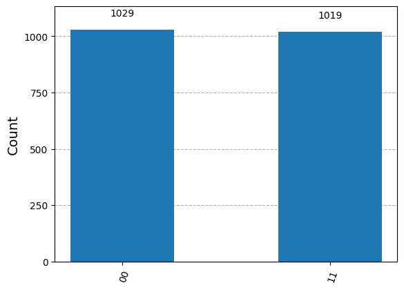
counts = simulate(qc_equiv)
plot_histogram(counts)

Pulse Sequence Program

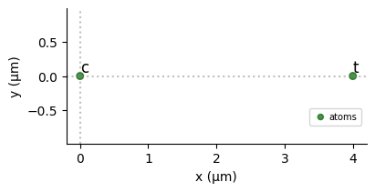
We begin by defining the qubits in a register. We’ll use two qubits labeled c and t respectively.

qubits = {
    'c': (0, 0),
    't': (4, 0)
}
reg = Register(qubits)
reg.draw()

Pulse

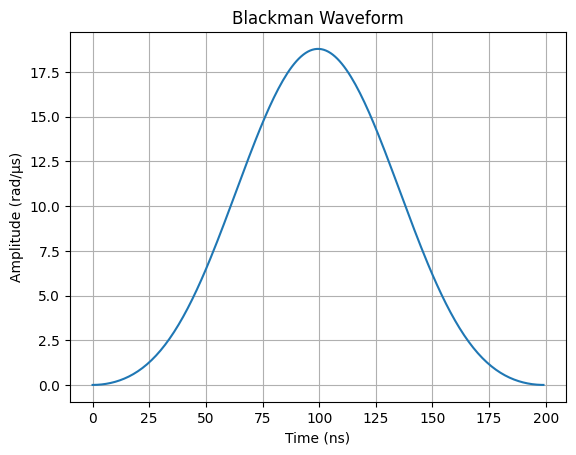
A pulse is a signal \(p: [T_1, T_2] \rightarrow \mathbb{R}\). One popular pulse is known as the Blackman waveform.

half_pi_wf = BlackmanWaveform(200, np.pi/2)
plt.plot(half_pi_wf.samples)
plt.title("Blackman Waveform")
plt.xlabel("Time (ns)")
plt.ylabel("Amplitude (rad/µs)")
plt.grid(True)

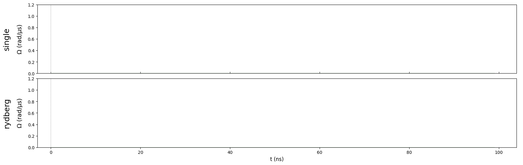
Pulse Sequence

A pulse sequence is a list of pulses. We’ll define two channels to accumulate pulse sequences using pulser.

1. The single channel will be used to accumulate pulses applied to single qubits.

2. The rydberg channel will be used to accumulate pulses applied to multiple qubits.

seq = Sequence(reg, DigitalAnalogDevice)
seq.declare_channel(
    'single',        # Name of channel
    'raman_local'    # Single qubit channel only requires raman component
)
seq.declare_channel(
    'rydberg',       # Name of channel
    'rydberg_local'  # Multi-qubit channel requires Rydberg Blockade
)
seq.draw(draw_phase_curve=True)

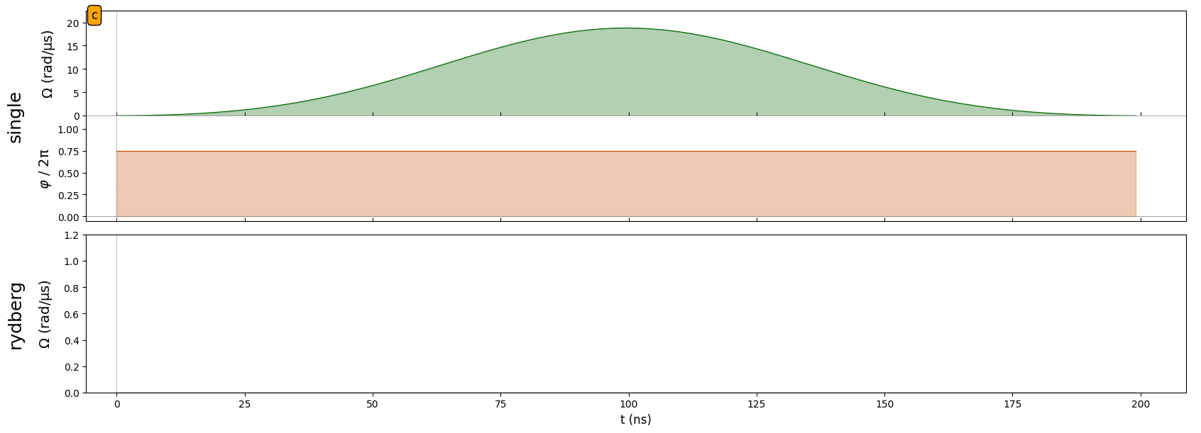
\(RY(\pi/2)\)

We can use our first pulse sequence to simulate a \(RY(\pi/2)\) gate.

ry_pulse = Pulse.ConstantDetuning(
    amplitude=half_pi_wf,
    detuning=0,
    phase=-np.pi/2,
)
seq.target('c', 'single')
seq.add(ry_pulse, 'single')
seq.draw(draw_phase_curve=True)

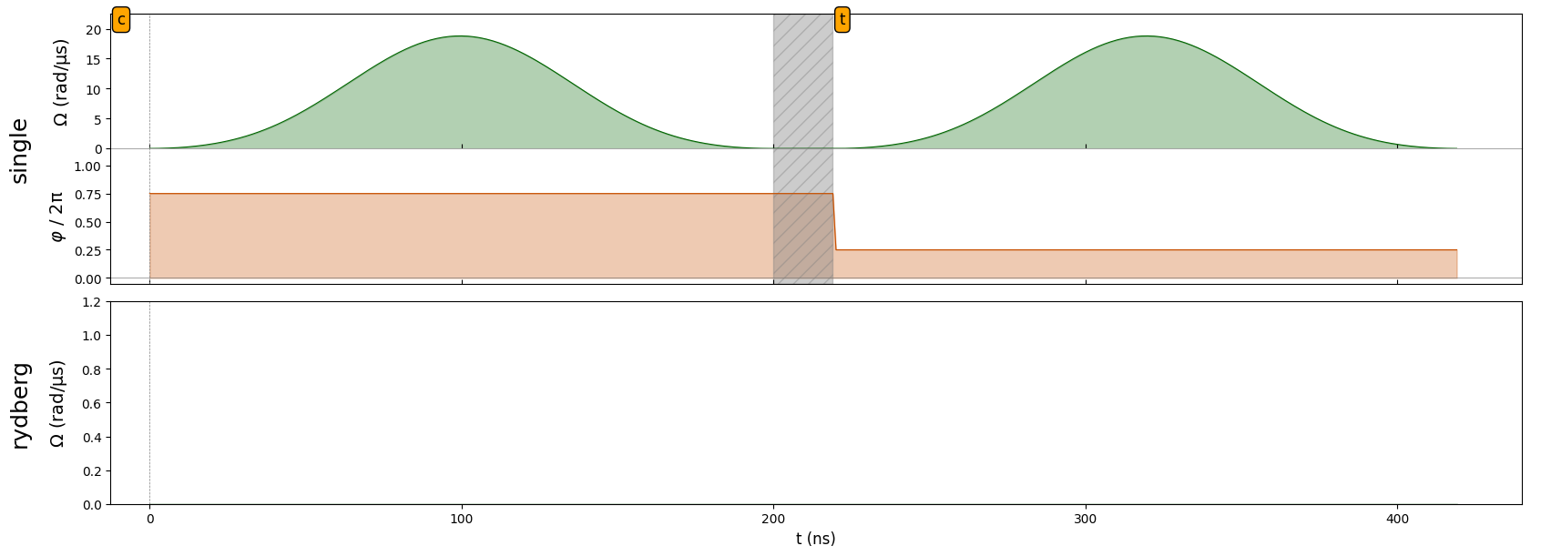
\(RY(-\pi/2)\)

We can also apply \(RY(-\pi/2)\) by changing the phase. Note that the qubit we are applying the qubit to is notated in the top-left.

ry_dag_pulse = Pulse.ConstantDetuning(
    amplitude=half_pi_wf,
    detuning=0,
    phase=np.pi/2,
)
seq.target('t', 'single')
seq.add(ry_dag_pulse, 'single')
seq.draw(draw_phase_curve=True)

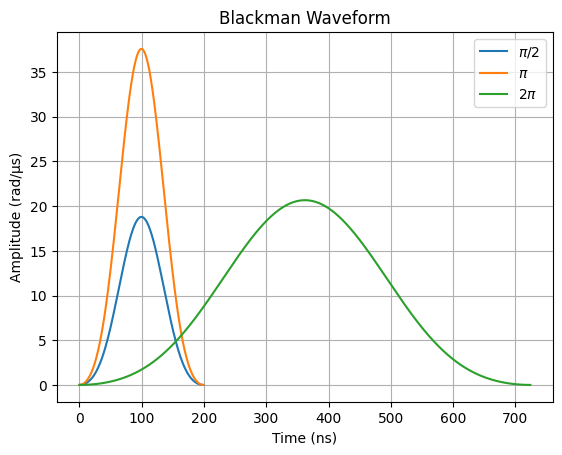
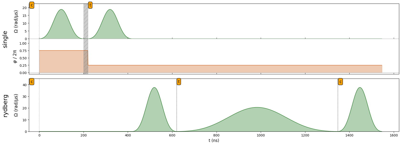
CZ Gate

We will now apply the sequence of pulses corresponding to a CZ gate. To accomplish this, we will need to use the Rydberg Blockade so that nearby atoms can interact and devise more pulses.

max_val = DigitalAnalogDevice.rabi_from_blockade(8)
max_val

20.67626392364502

pi_wf = BlackmanWaveform(200, np.pi)
two_pi_wf = BlackmanWaveform.from_max_val(
    max_val=max_val,
    area=2*np.pi,
)
plt.plot(half_pi_wf.samples, label=r"$\pi/2$")
plt.plot(pi_wf.samples, label=r"$\pi$")
plt.plot(two_pi_wf.samples, label=r"$2\pi$")
plt.title("Blackman Waveform")
plt.xlabel("Time (ns)")
plt.ylabel("Amplitude (rad/µs)")
plt.grid(True)
plt.legend();

seq.target('c', 'rydberg')
seq.align('single', 'rydberg')
pi_pulse = Pulse.ConstantDetuning(pi_wf, 0, 0)
seq.add(pi_pulse, 'rydberg')
two_pi_pulse = Pulse.ConstantDetuning(
    amplitude=two_pi_wf,
    detuning=0,
    phase=0,
)
seq.target('t', 'rydberg')
seq.add(two_pi_pulse, 'rydberg')
seq.target('c', 'rydberg')
seq.add(pi_pulse, 'rydberg')
seq.draw(draw_phase_curve=True)

/opt/hostedtoolcache/Python/3.12.6/x64/lib/python3.12/site-packages/pulser/sequence/sequence.py:1302: UserWarning: A duration of 725 ns is not a multiple of the channel's clock period (4 ns). It was rounded up to 728 ns.
  self._add(pulse, channel, protocol)

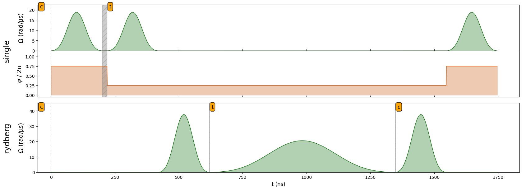
\(RY(\pi/2)\)

Finally, we apply the last \(RY(\pi/2)\) gate.

seq.align('single', 'rydberg')
seq.add(ry_pulse, 'single')
seq.draw(draw_phase_curve=True)

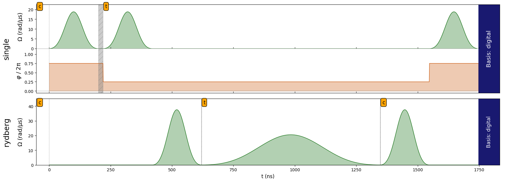
Measurement

seq.measure(basis='digital')
seq.draw(draw_phase_curve=True)

sim = QutipEmulator.from_sequence(seq)
res = sim.run()
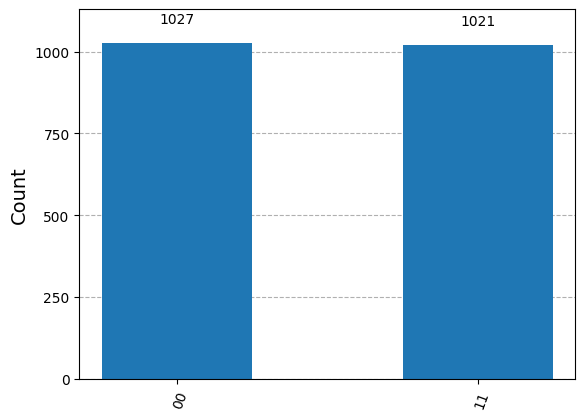
counts = res.sample_final_state(N_samples=2048)
plot_histogram(counts)

/opt/hostedtoolcache/Python/3.12.6/x64/lib/python3.12/site-packages/qutip/solver/options.py:16: FutureWarning: Dedicated options class are no longer needed, options should be passed as dict to solvers.
  warnings.warn(
/opt/hostedtoolcache/Python/3.12.6/x64/lib/python3.12/site-packages/qutip/solver/solver_base.py:459: FutureWarning: "progress_bar" is now included in options:
 Use `options={"progress_bar": False / True / "tqdm" / "enhanced"}`
  warnings.warn(

Summary

1. We saw how to program a neutral atom quantum computer with pulse sequences.

2. A pulse sequence gives fine-grained and analog control over the implementation of a digital gates.

3. We saw how to use the Rydberg blockade to implement a pulse sequence to implement the \(CZ\) gate.

References

[1] Pulser: An open-source package for the design of pulse sequences in programmable neutral-atom arraysm