from bloqade import start
from bloqade.constants import RB_C6
from qutip import sigmax, basis, mesolve, tensor, Qobj
import numpy as np

from util import zero, one, pretty, plot_histogram, histogram_final_state, invert_keys

Neutral Atom Quantum Computing

In this notebook, we will introduce Neutral Atom Quantum Computing. Neutral Atom QC uses properties of Rydberg atoms to implement quantum computations.

Rydberg Atoms

A Rydberg atom is any atom that has one or more excited electrons whose distance (on average) from the nucleus is large. This means that a Rydberg atom placed in proximity to another one can have excited electrons that can interact with another to exhibit quantum effects such as entanglement. The ground state of a Rydberg atom is notated \(\ket{g}\) and the excited state is notated \(\ket{r}\). We can encode

1. \(\ket{0} = \ket{g}\)

2. \(\ket{1} = \ket{r}\)

to perform quantum computations with Rydberg atoms.

Rubidium Atoms

The Aquila neutral atom quantum computer [3] [4] uses Rubidium (Rb37) atoms as its implementation of a Rydberg atom. In the example below, we have place 4 Rydberg atoms on a tabletop.

register = start.add_position([
    (0, 0), # 1
    (5, 0), # 2
    (0, 5), # 3
    (5, 5), # 4
])  # (um)
print(register)

                                   Atom Positions                               
    ┌──────────────────────────────────────────────────────────────────────────┐
5.00┤•                                                                        •│
    │                                                                          │
    │                                                                          │
4.17┤                                                                          │
    │                                                                          │
    │                                                                          │
3.33┤                                                                          │
    │                                                                          │
    │                                                                          │
2.50┤                                                                          │
    │                                                                          │
    │                                                                          │
1.67┤                                                                          │
    │                                                                          │
    │                                                                          │
0.83┤                                                                          │
    │                                                                          │
    │                                                                          │
0.00┤•                                                                        •│
    └┬─────────────────┬──────────────────┬─────────────────┬─────────────────┬┘
    0.0               1.2                2.5               3.8              5.0 
y (um)                                 x (um)                                   

In the above, we have 4 Rydberg atoms

\[ \ket{\psi} = \ket{q_4 q_3 q_2 q_1} \,. \]

Rydberg Hamiltonian

Rydberg atoms are governed by the Rydberg Hamiltonian. We’ll begin with a 1 qubit example of a Rydberg Hamiltonian before working our way to the general case.

Single Qubit

The Rydberg Hamiltonian on a single qubit (i.e., Rydberg atom) is given as

\[\begin{align*} \frac{1}{\hbar} H_{\text{Rydberg}}(t) & = \underbrace{\frac{\Omega(t)}{2} \begin{pmatrix} 0 & e^{i\phi(t)} \\ e^{-i\phi(t)} & 0 \end{pmatrix}}_{H_\text{couple}} - \underbrace{\begin{pmatrix} 0 & 0 \\ 0 & \Delta(t) \end{pmatrix}}_{{H_\text{detune}}} \\ & = \begin{pmatrix} 0 & \frac{\Omega(t)}{2} e^{i\phi(t)} \\ \frac{\Omega(t)}{2} e^{-i\phi(t)} & -\Delta(t) \end{pmatrix} \end{align*}\]

where

1. \(\Omega(t)\) is a Rabi frequency,

2. \(\phi(t)\) is the Rabi phase, and

3. \(\Delta(t)\) is the detuning of the driving laser.

def H_couple1(Omega, phi, t):
    return Omega(t)/2 * Qobj(np.array([
        [0.0, np.exp(1j * phi(t))],
        [np.exp(-1j * phi(t)), 0.0],
    ]))

def H_detune1(Delta, t):
    return Qobj(np.array([
        [0.0, 0.0],
        [0.0, Delta(t)],
    ]))

def H_rydberg1(Omega, phi, Delta, t):
    return H_couple1(Omega, phi, t) - H_detune1(Delta, t)

Pauli-X Gate

We can encode a Pauli-X gate with a Rydberg Hamiltonian.

Omega = lambda t: 2
phi = lambda t: 0
Delta = lambda t: 0

sigma_x = H_rydberg1(Omega, phi, Delta, 0)
pretty(sigma_x.full())

\[\begin{split}\begin{bmatrix} 0 & 1 \\ 1 & 0 \\ \end{bmatrix} \end{split}\]

Notice that we have recreated the Hamiltonian for a Pauli-X (up to a scale).

pretty(sigmax().full())

\[\begin{split}\begin{bmatrix} 0 & 1 \\ 1 & 0 \\ \end{bmatrix} \end{split}\]

RX_gate = (-1j * sigma_x * np.pi/2).expm()
pretty(RX_gate.full())

\[\begin{split}\begin{bmatrix} 0 & - i \\ - i & 0 \\ \end{bmatrix} \end{split}\]

We can adjust the phase picked up by the Hamiltonian by adjusting \(\phi\).

Omega = lambda t: 2
phi = lambda t: 3*np.pi/2
Delta = lambda t: 0

X = H_rydberg1(Omega, phi, Delta, 0)
pretty(X.full())

\[\begin{split}\begin{bmatrix} 0 & - i \\ i & 0 \\ \end{bmatrix} \end{split}\]

Bloqade

Bloqade gives us a Python interface to neutral atom quantum hardware. We can write a program for neutral atom quantum hardware by writing down the Rydberg Hamiltonian. To do this, we specify qubits by placing them on \((x, y)\) locations on a 2D plane. We then control the computation by specifying \(\Omega(t)\), \(\phi(t)\), and \(\Delta(t)\) as waveforms that encode the time-dependent signals.

T = np.pi
register = start.add_position([(0, 0)])  # (um)
program = (
    register
    .rydberg.rabi.amplitude.uniform.piecewise_constant( # Omega = lambda t: 15
        durations=[T],
        values=[15]
    )
    .rydberg.rabi.phase.uniform.piecewise_constant( # phi = lambda t: 0
        durations=[T],
        values=[0]
    )
    .rydberg.detuning.uniform.piecewise_constant( # Delta = lambda t: 0
        durations=[T],
        values=[0]
    )
)
print(program)

Routine
                                   Atom Positions                               
     ┌─────────────────────────────────────────────────────────────────────────┐
 1.00┤                                                                         │
     │                                                                         │
     │                                                                         │
 0.67┤                                                                         │
     │                                                                         │
     │                                                                         │
 0.33┤                                                                         │
     │                                                                         │
     │                                                                         │
 0.00┤                                    •                                    │
     │                                                                         │
     │                                                                         │
-0.33┤                                                                         │
     │                                                                         │
     │                                                                         │
-0.67┤                                                                         │
     │                                                                         │
     │                                                                         │
-1.00┤                                                                         │
     └┬─────────────────┬─────────────────┬─────────────────┬─────────────────┬┘
    -1.00             -0.50             0.00              0.50             1.00 
y (um)                                 x (um)                                   

Sequence
└─ RydbergLevelCoupling
   ⇒ Pulse
     ├─ RabiFrequencyAmplitude
     │  ⇒ Field
     │    └─ Drive
     │       ├─ modulation
     │       │  ⇒ UniformModulation
     │       └─ waveform
     │          ⇒ Constant
     │            ├─ value
     │            │  ⇒ Literal: 15
     │            └─ duration
     │               ⇒ Literal: 3.141592653589793
     ├─ RabiFrequencyPhase
     │  ⇒ Field
     │    └─ Drive
     │       ├─ modulation
     │       │  ⇒ UniformModulation
     │       └─ waveform
     │          ⇒ Constant
     │            ├─ value
     │            │  ⇒ Literal: 0
     │            └─ duration
     │               ⇒ Literal: 3.141592653589793
     └─ Detuning
        ⇒ Field
          └─ Drive
             ├─ modulation
             │  ⇒ UniformModulation
             └─ waveform
                ⇒ Constant
                  ├─ value
                  │  ⇒ Literal: 0
                  └─ duration
                     ⇒ Literal: 3.141592653589793
---------------------
> Static params:

> Batch params:
- batch 0:

> Arguments:
  ()

results = program.bloqade.python().run(1000)
report = results.report()
invert_keys(report.counts())

[OrderedDict([('1', 1000)])]

General Case

The Rydberg Hamiltonian in the general case is given as

\[ \frac{H(t)}{\hbar} = H_\text{coupling} - H_\text{detune} + H_\text{interaction}\,. \]

Compared to the single qubit case, we will have a generalization of \(H_\text{coupling}\) and \(H_\text{detune}\) as well as an additional term \(H_\text{interaction}\) that will enable us to entangle qubits. We’ll go over each term now.

Coupling Term

The term

\[ H_\text{coupling} = \frac{\Omega(t)}{2} \sum_{j=1}^n (e^{i\phi_j(t)} |g_j\rangle\langle r_j| + e^{-i\phi_j(t)} |r_j\rangle\langle g_j|) \]

decribes the strength of the coupling between the ground state \(\ket{g_j}\) and the excited state \(\ket{r_j}\).

1. The notation \(|g_j\rangle \langle r_j| = I(j-1) \otimes |g\rangle\langle r| \otimes I(n - j - 1)\) selects the \(j\)-th qubit.

2. \(\Omega_j(t)\) gives the Rabi frequency as a function of time.

3. \(\phi_j(t)\) gives the Rabi phase as a function of time.

def mk_H_couple(n, Omega, phi):
    sigma_x = Omega / 2 * (np.exp(1j * phi) * np.outer(zero, one) + np.exp(-1j * phi) * np.outer(one, zero))
    H = np.zeros((2**n, 2**n), dtype=np.complex128)
    for j in range(n):
        if j == 0:
            H += np.kron(sigma_x, np.eye(2**(n-1)))
        elif j == n - 1:
            H += np.kron(np.eye(2**(n-1)), sigma_x)
        else:
            H += np.kron(np.eye(2**j), np.kron(sigma_x, np.eye(2**(n-j-1))))
    return H

Omega = 15
phi = 0
H_couple = mk_H_couple(2, Omega, phi)
pretty(H_couple)

\[\begin{split}\begin{bmatrix} 0 & \frac{15}{2} & \frac{15}{2} & 0 \\ \frac{15}{2} & 0 & 0 & \frac{15}{2} \\ \frac{15}{2} & 0 & 0 & \frac{15}{2} \\ 0 & \frac{15}{2} & \frac{15}{2} & 0 \\ \end{bmatrix} \end{split}\]

Coupling as \(\sigma_x\)

We can rewrite

\[ H_\text{coupling} = \frac{\Omega(t)}{2} \sum_{j=1}^n \sigma_x^j |g_j\rangle\langle r_j| \]

where

1. \(\sigma_x^j\) is the Pauli-X gate applied to the \(j\)-th qubit and

2. \(|g_j\rangle \langle r_j| = I(j-1) \otimes |g\rangle\langle r| \otimes I(n - j - 1)\) selects the \(j\)-th qubit.

Thus we can think of the coupling term as applying \(\sigma_x\) to each qubit.

Detuning Term

The detuing term is defined as

\[ H_\text{detune} = -\Delta(t) \sum_{j=1}^n \hat{n}_j \]

where \(\hat{n}_j = |r_j\rangle\langle r_j|\) is the number operator.

def nhats(n: int, j: int) -> np.ndarray:
    oo_op = np.outer(one, one)
    if j == 0:
        return np.kron(oo_op, np.eye(2**(n-1)))
    elif j == n - 1:
        return np.kron(np.eye(2**(n-1)), oo_op)
    else:
        return np.kron(np.eye(2**j), np.kron(oo_op, np.eye(2**(n-j-1))))

def mk_H_detune(n: int, Delta: float) -> np.ndarray:
    H = np.zeros((2**n, 2**n), dtype=np.complex128)
    for j in range(n):
        H += nhats(n, j)
    return Delta * H
    
# Detune
Delta = -15
H_detune = mk_H_detune(2, Delta)
pretty(H_detune)

\[\begin{split}\begin{bmatrix} 0 & 0 & 0 & 0 \\ 0 & -15 & 0 & 0 \\ 0 & 0 & -15 & 0 \\ 0 & 0 & 0 & -30 \\ \end{bmatrix} \end{split}\]

Van-dar Waals Interaction Term

The final term is the interaction term

\[ H_\text{interaction} = \sum_{j < k} V_{jk} \hat{n}_j\hat{n}_k \]

where

\[ V_{jk} = \frac{C_6}{|x_j - x_K|^6} \]

and \(x_j\) and \(x_k\) are atom positions. This term, when combined with the phenomenon of the Rydberg bloqade, is what enables us to create entangled qubits.

register = start.add_position([
    (0, 0), # (um)
    (5, 0)  # (um)
])
print(register)

                                   Atom Positions                               
     ┌─────────────────────────────────────────────────────────────────────────┐
 1.00┤                                                                         │
     │                                                                         │
     │                                                                         │
 0.67┤                                                                         │
     │                                                                         │
     │                                                                         │
 0.33┤                                                                         │
     │                                                                         │
     │                                                                         │
 0.00┤•                                                                       •│
     │                                                                         │
     │                                                                         │
-0.33┤                                                                         │
     │                                                                         │
     │                                                                         │
-0.67┤                                                                         │
     │                                                                         │
     │                                                                         │
-1.00┤                                                                         │
     └┬─────────────────┬─────────────────┬─────────────────┬─────────────────┬┘
     0.0               1.2               2.5               3.8              5.0 
y (um)                                 x (um)                                   

V_jk = register.rydberg_interaction()
V_jk

array([[  0.        ,   0.        ],
       [346.90823249,   0.        ]])

def interaction_strength(x, y):
    return RB_C6 / np.linalg.norm((x - y)) ** 6

interaction_strength(np.array([0, 0]), np.array([5, 0]))

346.90823248964847

def mk_H_interaction(n, register):
    V_jk = register.rydberg_interaction()
    H_interaction = np.zeros((2**n, 2**n), dtype=np.complex128)
    for row in range(0, n):
        for col in range(0, row+1):
            if row != col:
                print(row, col)
                H_interaction += V_jk[row, col] * nhats(n, col) @ nhats(n, row)
    return H_interaction

H_interaction = mk_H_interaction(2, register)
pretty(H_interaction)

1 0

\[\begin{split}\begin{bmatrix} 0 & 0 & 0 & 0 \\ 0 & 0 & 0 & 0 \\ 0 & 0 & 0 & 0 \\ 0 & 0 & 0 & 346.9082324896 \\ \end{bmatrix} \end{split}\]

Putting it together

We can finally put together the Rydberg Hamiltonian

\[ \frac{H(t)}{\hbar} = H_\text{coupling} - H_\text{detune} + H_\text{interaction}\,. \]

def mk_H_Rydberg(n, Omega, phi, Delta, register):
    H_couple = mk_H_couple(n, Omega, phi)
    H_detune = mk_H_detune(n, Delta)
    H_interaction = mk_H_interaction(n, register)
    return H_couple - H_detune + H_interaction

H_rydberg = mk_H_Rydberg(2, Omega, phi, Delta, register)
pretty(H_rydberg)

1 0

\[\begin{split}\begin{bmatrix} 0 & \frac{15}{2} & \frac{15}{2} & 0 \\ \frac{15}{2} & 15 & 0 & \frac{15}{2} \\ \frac{15}{2} & 0 & 15 & \frac{15}{2} \\ 0 & \frac{15}{2} & \frac{15}{2} & 376.9082324896 \\ \end{bmatrix} \end{split}\]

Two Qubit Case

Written out, the two qubit case is

\[\begin{align*} \frac{1}{\hbar} H_{\text{Rydberg}}(t) & = \underbrace{\begin{pmatrix} 0 & \frac{\Omega_2(t)}{2} e^{i\phi_2(t)} & \frac{\Omega_1(t)}{2} e^{i\phi_1(t)} & 0 \\ \frac{\Omega_2(t)}{2} e^{-i\phi_2(t)} & 0 & 0 & \frac{\Omega_1(t)}{2} e^{i\phi_1(t)} \\ \frac{\Omega_1(t)}{2} e^{-i\phi_1(t)} & 0 & 0 & \frac{\Omega_2(t)}{2} e^{i\phi_2(t)} \\ 0 & \frac{\Omega_1(t)}{2} e^{-i\phi_1(t)} & \frac{\Omega_2(t)}{2} e^{-i\phi_2(t)} & 0 \end{pmatrix}}_{H_\text{couple}} + \\ & \phantom{=} \underbrace{\begin{pmatrix} 0 & 0 & 0 & 0 \\ 0 & \Delta_2(t) & 0 & 0 \\ 0 & 0 & \Delta_1(t) & 0 \\ 0 & 0 & 0 & \Delta_1(t) + \Delta_2(t) \end{pmatrix}}_{H_\text{detune}} + \underbrace{\begin{pmatrix} 0 & 0 & 0 & 0 \\ 0 & 0 & 0 & 0 \\ 0 & 0 & 0 & 0 \\ 0 & 0 & 0 & V_{1,2} \end{pmatrix}}_{H_\text{interaction}} \\ & = \begin{pmatrix} 0 & \frac{\Omega_2(t)}{2} e^{i\phi_2(t)} & \frac{\Omega_1(t)}{2} e^{i\phi_1(t)} & 0 \\ \frac{\Omega_2(t)}{2} e^{-i\phi_2(t)} & \Delta_2(t) & 0 & \frac{\Omega_1(t)}{2} e^{i\phi_1(t)} \\ \frac{\Omega_1(t)}{2} e^{-i\phi_1(t)} & 0 & \Delta_1(t) & \frac{\Omega_2(t)}{2} e^{i\phi_2(t)} \\ 0 & \frac{\Omega_1(t)}{2} e^{-i\phi_1(t)} & \frac{\Omega_2(t)}{2} e^{-i\phi_2(t)} & \Delta_1(t) + \Delta_2(t) + V_{1,2} \end{pmatrix} \end{align*}\]

Bloqade Simulation

We can simulate the Rydberg Hamiltonian using Bloqade.

def simple_prog(register, T=np.pi/2):
    program = (
        register
        .rydberg.rabi.amplitude.uniform.piecewise_constant( # Omega = lambda t: 15
            durations=[T],
            values=[15]
        )
        .rydberg.rabi.phase.uniform.piecewise_constant( # phi = lambda t: 0
            durations=[T],
            values=[0]
        )
        .rydberg.detuning.uniform.piecewise_constant( # Delta = lambda t: 0
            durations=[T],
            values=[0]
        )
    )
    return program

register = start.add_position([(0,0), (5,0)])  # (um)
results = simple_prog(register).bloqade.python().run(2048)
report = results.report()
plot_histogram(invert_keys(report.counts()))

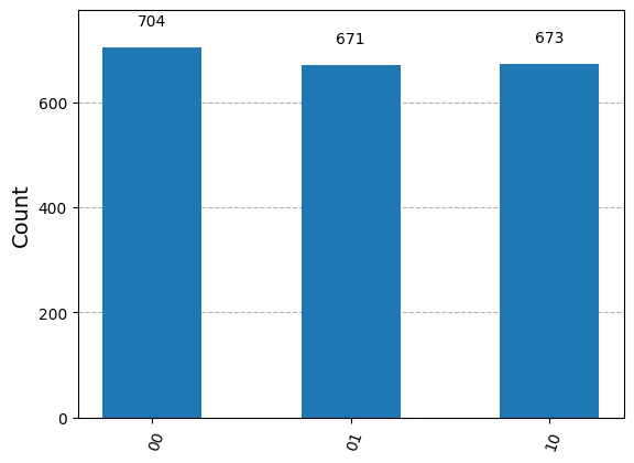
Rydberg Blockade

The Rydberg Blockade is a phenomenon where an excited state of one qubit prevents another nearby qubit from being excited, thus producing the effect of entanglement. In the example above, we “rarely” observed the outcome \(\ket{11}\) due to the blockade mechanism. Mathematically, we saw that the distance between the atoms affected the Hamiltonian through the interaction term. The blockade radius is defined as

\[ R_\text{blockade} = \left( \frac{C_6}{\Omega} \right)^{1/6} \,. \]

When the distance between two atoms is less than \(R_\text{blockade}\), the excited state of one atom will block the other from getting excited. Outside of \(R_\text{blockade}\), each atom will have less and less of an effect.

def bloqade_radius(Omega):
    return (RB_C6 / Omega) ** (1/6)

print("Bloqade radius", bloqade_radius(Omega), "um")

Bloqade radius 8.439639489080086 um

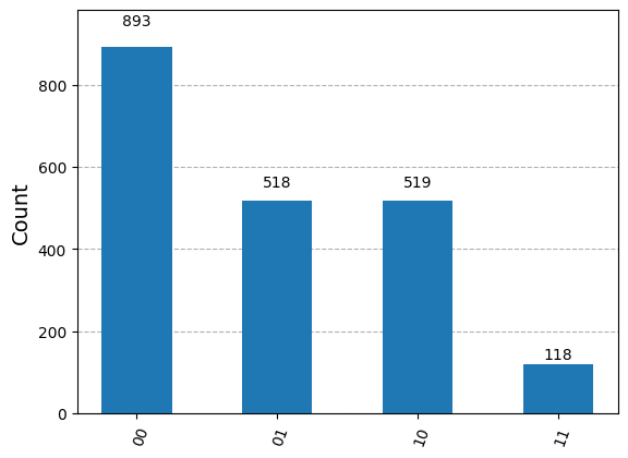
Outside of blockade radius

register = start.add_position([(0,0), (8.7, 0)])  # (um)
results = simple_prog(register).bloqade.python().run(2048)
report = results.report()
plot_histogram(invert_keys(report.counts()))

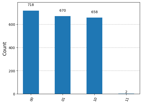
Within blockade radius

register = start.add_position([(0,0), (8.42, 0)])  # (um)
results = simple_prog(register).bloqade.python().run(2048)
report = results.report()
plot_histogram(invert_keys(report.counts()))

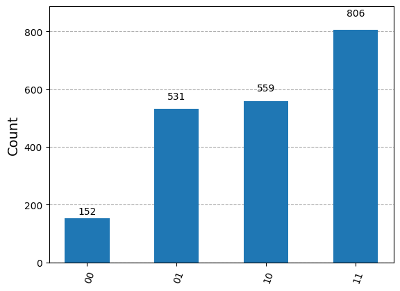
Qutip Simulation

As before, we can also use qutip to solve Schrödinger’s equation.

T = np.pi/2
times = np.linspace(0, T, 100)
register = start.add_position([(0,0), (5,0)])  # (um)
H_rydberg = mk_H_Rydberg(2, Omega, phi, Delta, register)
z = basis(2, 0)
result = mesolve(Qobj(H_rydberg, dims=[[2, 2], [2, 2]]), tensor(z, z), times, [], [])
pretty(result.final_state)

1 0

\[(-0.3993257718 + 0.4267773594 i) |00\rangle+(0.4915346683 - 0.2955074189 i) |01\rangle+(0.4915346683 - 0.2955074189 i) |10\rangle+(-0.0203321842 + 0.0111662989 i) |11\rangle\]

plot_histogram(histogram_final_state(result.final_state.full()))

Summary

1. We introduced neutral atom quantum computing based on Rydberg atoms.

2. We introduced the Rydberg Hamiltonian and gave a few examples.

3. We examined the Rydberg Blockade mechanism which enables nearby qubits to interact with each other.

References

[1] Rydberg Hamiltonian

[2] Rydberg Blockade

[3] https://bloqade.quera.com/0.15.14/

[4] https://www.quera.com/glossary/rubidium