import numpy as np
import matplotlib.pyplot as plt
from typing import *

from qiskit_aer import AerSimulator
from qiskit.quantum_info import Statevector
from qiskit.visualization import plot_bloch_multivector
sim = AerSimulator()

from util import zero, one, demonstrate_measure

Foundations: Bloch Spheres: Visualization for Single Qubit

In this notebook, we’ll continue our exploration of a single qubit system by introducing the Bloch sphere, a visual representation of a single qubit.

References

1. Introduction to Classical and Quantum Computing: Chapter 2

Bloch Sphere

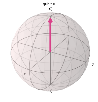
1. A Bloch sphere enables us to visualize the quantum state of a single qubit.

2. This visualization will enable us to introduce operations on single qubits geometrically as transformations on the Bloch sphere.

plot_bloch_multivector(zero)

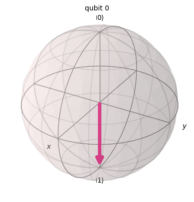
plot_bloch_multivector(one)

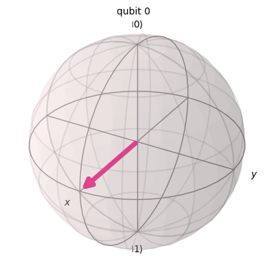
Visualizing Superposition

Every point on the surface of the Bloch sphere encodes a valid quantum state for a single qubit system. This graphically shows that there are an infinite number of quantum states that can be represented by a single qubit. Any qubit that is not at the north or south pole of the Bloch sphere is then in superposition.

q1 = 1/np.sqrt(2)*zero + 1/np.sqrt(2)*one 
q1.draw('latex')

\[\frac{\sqrt{2}}{2} |0\rangle+\frac{\sqrt{2}}{2} |1\rangle\]

plot_bloch_multivector(q1)

Note

1. A state in superposition is a single quantum state.

2. It happens to be a “mixture” of the \(|0\rangle\) and \(|1\rangle\) state.

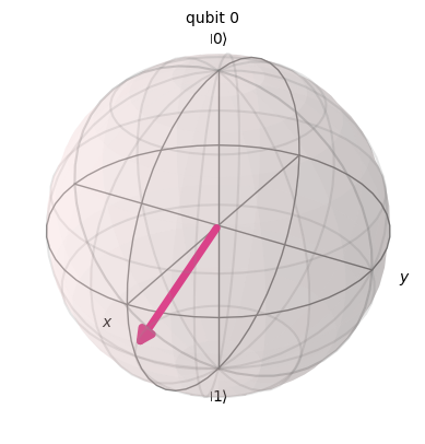
q2 = np.sqrt(1/3)*zero + np.sqrt(2/3)*one
Statevector(q2).draw('latex')

\[\frac{\sqrt{3}}{3} |0\rangle+\frac{\sqrt{6}}{3} |1\rangle\]

plot_bloch_multivector(q2)

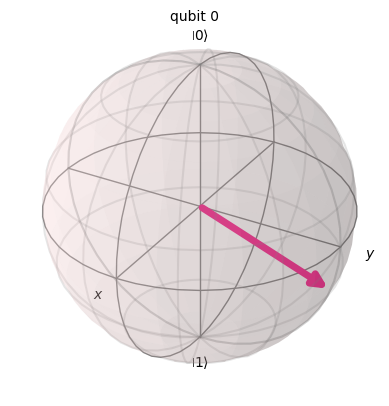
q3 = np.sqrt(-1/3*1j)*zero + np.sqrt(2/3*1j)*one
Statevector(q3).draw('latex')

\[(\frac{\sqrt{6}}{6} - \frac{\sqrt{6} i}{6}) |0\rangle+(\frac{\sqrt{3}}{3} + \frac{\sqrt{3} i}{3}) |1\rangle\]

plot_bloch_multivector(q3)

Translating to a Bloch Sphere

Every qubit \(|q\rangle \in Q(1)\) can be written as

\[ |q\rangle = \cos \frac{\theta}{2} |0\rangle + e^{i\phi}\sin \frac{\theta}{2} |1\rangle \]

where

1. \(0 \leq \theta \leq \pi\) is the polar angle (\(\theta = 0\) means \(|0\rangle\) is north and \(\theta = \pi\) means \(|1\rangle\) is south) and

2. \(0 \leq \phi \leq 2\pi\) is the azimuthal angle.

Aside 1: Euler’s Formula

The complex exponential \(e^{i\phi}\) is defined as

\[ e^{i\phi} = cos \phi + i sin \phi \,. \]

This is known as Euler’s formula.

np.exp(np.deg2rad(30)*1j)

np.complex128(0.8660254037844387+0.49999999999999994j)

np.cos(np.deg2rad(30)) + np.sin(np.deg2rad(30))*1j

np.complex128(0.8660254037844387+0.49999999999999994j)

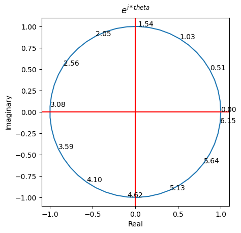
Graphical interpretation of Euler’s formula

1. As a reminder, every operation on complex numbers can be visualized on the complex plane.

2. Euler’s formula corresponds to the unit circle on the complex plane.

fig = plt.figure(); ax = fig.add_subplot()
ax.set_aspect(1.0/ax.get_data_ratio(), adjustable='box')

# Plot
thetas = np.linspace(0, 2*np.pi)                 # 50 evenly spaces points in [0, 2\pi]
txt = [f"{theta:.2f}" for theta in thetas]
zs = [np.exp(theta * 1j) for theta in thetas]    # e^(j\theta) or e^(i\theta) for theta in [0, 2\pi]
for i, t in enumerate(txt):
    if i % 4 == 0:
        plt.annotate(t, (zs[i].real, zs[i].imag))

# Plot meta-data
plt.plot([z.real for z in zs], [z.imag for z in zs])
plt.axhline(y=0.0, color='r', linestyle='-'); plt.axvline(x=0.0, color='r', linestyle='-')
plt.xlabel('Real'); plt.ylabel('Imaginary'); plt.title('$e^{i * theta}$')

Text(0.5, 1.0, '$e^{i * theta}$')

Example: Translating to a Bloch Sphere

We give an example translation now (Following [1]). For reference, the formula is

\[ |q\rangle = \cos \frac{\theta}{2} |0\rangle + e^{i\phi}\sin \frac{\theta}{2} |1\rangle \,. \]

q2.draw('latex')

\[\frac{\sqrt{3}}{3} |0\rangle+\frac{\sqrt{6}}{3} |1\rangle\]

Observations

Observe that

\[ \frac{\sqrt{3}}{3} = \cos(\theta/2) \]

and

\[ \frac{\sqrt{6}}{3} = e^{i\phi} \sin(\theta/2) \,. \]

def convert_alpha(alpha: float) -> float:
    return 2*np.rad2deg(np.arccos(alpha))

theta = convert_alpha(np.sqrt(3)/3)
theta

np.float64(109.47122063449069)

# Check conversion of alpha
print("Original coefficient", np.sqrt(3)/3)
print("From calculation", np.cos(np.deg2rad(theta)/2))

Original coefficient 0.5773502691896257
From calculation 0.5773502691896257

# Check conversion of beta which is missing a factor of e^{i\phi}
np.sin(np.deg2rad(theta)/2), np.sqrt(6)/3

(np.float64(0.816496580927726), np.float64(0.8164965809277259))

# Can infer that phi is 0
phi = 0
phi, np.exp(0j)

(0, np.complex128(1+0j))

plot_bloch_multivector(q2)

Aside 2: Global Phase

1. The translation to a Bloch sphere might appear strange.

2. In particular, a pair of complex numbers is specified by 4 numbers subject to a constraint. This means that there are effectively only 3 numbers used to specify a point on the Bloch sphere.

3. However, the specification of a Bloch sphere only has 2 numbers!

4. The missing degree of freedom is called the global phase. The global phase is physically irrelevant.

q3.draw('latex')

\[(\frac{\sqrt{6}}{6} - \frac{\sqrt{6} i}{6}) |0\rangle+(\frac{\sqrt{3}}{3} + \frac{\sqrt{3} i}{3}) |1\rangle\]

Factor out global phase

def to_polar(z: np.complex128) -> Tuple[float, float]:
    r = np.linalg.norm(z)
    theta = np.rad2deg(np.arccos((z.real/r)))
    return r, theta

r0, theta0 = to_polar(q3[0])
print("r0", r0, "theta0", theta0)
r1, theta1 = to_polar(q3[1])
print("r1", r1, "theta1", theta1)

r0 0.5773502691896257 theta0 45.0
r1 0.816496580927726 theta1 45.00000000000001

(1)\[\begin{align} (\frac{\sqrt{6}}{6} - \frac{\sqrt{6}}{6}i) |0\rangle + (\frac{\sqrt{3}}{3} - \frac{\sqrt{3}}{3}i) |1\rangle & = e^{45\pi/180 i}\frac{\sqrt{3}}{3}|0\rangle + e^{45\pi/180 i}\frac{\sqrt{6}}{3}|1\rangle \tag{to polar} \\ & = e^{45\pi/180 i} (\frac{\sqrt{3}}{3}|0\rangle + \frac{\sqrt{6}}{3}|1\rangle) \tag{factor} \end{align}\]

1. The global phase is \(45^\circ\).

2. The relative phase is \(0^\circ\).

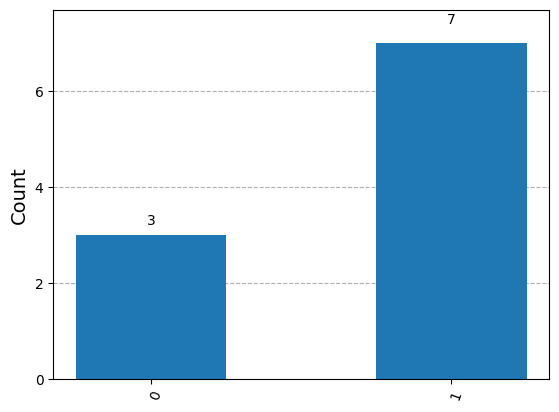
Global phase is indistinguishable by measurement

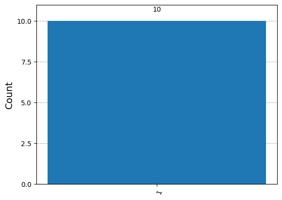
1. We have just seen that \(|q_2\rangle\) and \(|q_3\rangle\) are the same up to global phase.

2. This means that these two quantum states are indistinguishable by measurement.

3. We can see this since rotation by \(\phi\) on the Bloch sphere preserves the distance of the qubit encoding from \(|0\rangle\) to \(|1\rangle\) so that the probability of measurement is also preserved.

demonstrate_measure(q2)

demonstrate_measure(q3)

Summary

1. A Bloch sphere encodes the quantum state of a qubit up to global phase.

2. The global phase is indistinguishable by measurement.

3. The relative phase is given by \(\phi\) and is distinguishable.