import matplotlib.pyplot as plt
import numpy as np
import pandas as pd
from typing import *

from qiskit import transpile, QuantumCircuit, QuantumRegister, ClassicalRegister
from qiskit.quantum_info import Statevector, Operator
from qiskit.visualization import plot_histogram
from qiskit_aer import AerSimulator
sim = AerSimulator()

from util import zero, one, qft, amod15

Shor’s Part 4/5: Quantum Phase Estimation

Quantum phase estimation is an algorithm which when given a unitary matrix \(U\) and an eigenvector \(|u\rangle\), will produce the eigenvalue, i.e., the given phase \(e^{2\pi i \phi}\).

References

1. Introduction to Classical and Quantum Computing, Chapter 7.7 - 7.10

2. https://qiskit.org/textbook/ch-algorithms/shor.html

3. https://qiskit.org/textbook/ch-algorithms/quantum-phase-estimation.html

4. Introduction to Quantum Information Science: Lectures 20 and 21 by Scott Aaronson

5. Quantum Computation and Quantum Information: Chapter 5, Nielsen and Chuang

Building Blocks

QPE relies on two building blocks.

1. The first building block is a controlled-U operator which is a generalization of a controlled-NOT gate to an arbitrary unitary matrix \(U\).

2. The second building block is the inverse QFT which is the inverse of the QFT.

Algorithm Walkthrough

Suppose we are working with \(n\) bits. In RSA, we would have \(n = \log(N) = pq\). Then the QPE algorithm consts of the following steps.

1. Initialize state \(|u\rangle \otimes |0\rangle^{\otimes n}\) (little Endian) so that we have two registers of n bits.

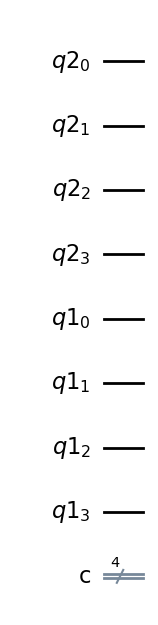
We’ll walkthrough the QPE algorithm using \(n = 4\) now.

n_count = 4
f_qc_U = lambda q: amod15(7, q)
reg1_size = f_qc_U(0).num_qubits

reg1 = QuantumRegister(reg1_size, "q1")
reg2 = QuantumRegister(n_count, "q2")
output = ClassicalRegister(n_count, "c")

# qc = QuantumCircuit(n_count+reg1_size, n_count)
qc = QuantumCircuit(reg2, reg1, output)
qc.draw(output="mpl", style="iqp")

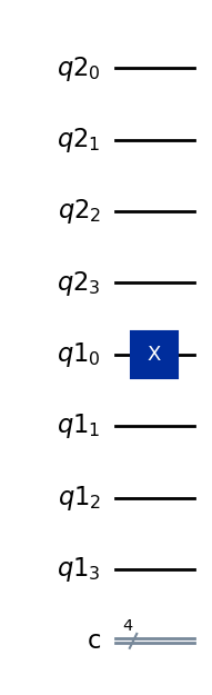
Step 1

Initialize state \(|u\rangle \otimes |0\rangle^{\otimes n}\) (little Endian) so that we have two registers of n bits.

# Step 1: Prepare our eigenstate |1>:
qc.x(n_count)
qc.draw(output="mpl", style="iqp")

State after Step 1

\[\begin{align*} |\psi_1\rangle & = (I^{\otimes 3} \otimes X \otimes I^{\otimes 4})|00000000\rangle \\ & = |00010000\rangle \end{align*}\]

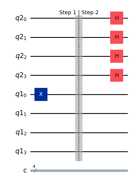
Step 2

Apply \(H^{\otimes t}\) to the first register.

# Step 2: Apply H-Gates to counting qubits.
qc.barrier(label="Step 1 | Step 2")
for qubit in range(n_count):
    qc.h(qubit)
qc.draw(output="mpl", style="iqp")

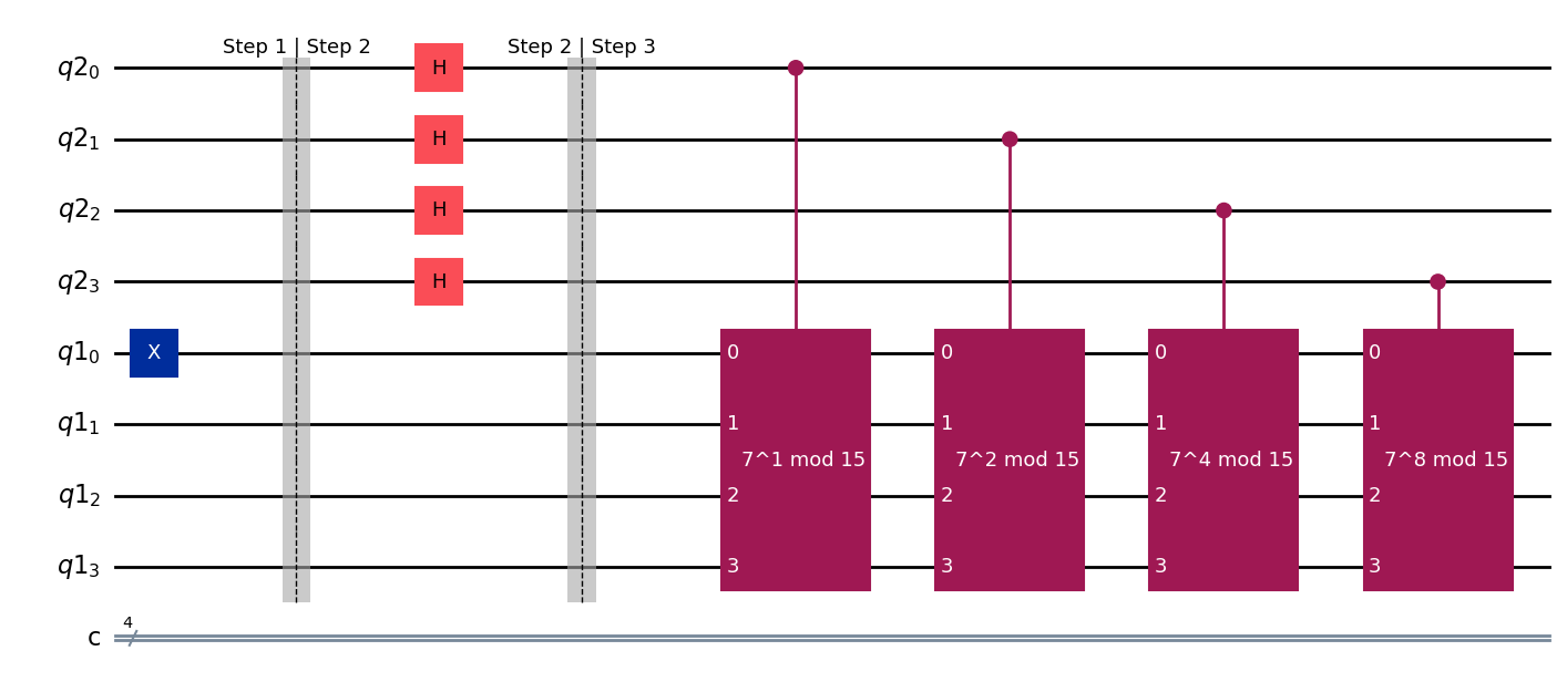
State after Step 2

\[\begin{align*} |\psi_2\rangle & = (I^{\otimes 4} \otimes H^{\otimes 4})|\psi_1\rangle \\ & = (I^{\otimes 4} \otimes H^{\otimes 4})|00010000\rangle \\ & = |0001++++\rangle \end{align*}\]

Step 3

Apply the controlled-U operator with control on the second register and targetting the first register.

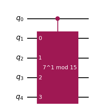
Controlled U Operator

1. As a reminder, a controlled not gate \(CNOT\) is a two-qubit gate that applies a not to the target qubit if the control qubit is set.

2. Similarly, a controlled \(U^{2^t \times 2^t}\) operator is a \(1+t\) qubit gate that applies \(U\) to \(t\) qubits if the control qubit is set.

qc_cu = QuantumCircuit(1 + 4)
a = 7; q = 0
qc_cu.append(
    amod15(a, 2**q).control(),
    # [q] is control
    # [1+i for i in range(4)] is target
    [q] + [1+i for i in range(4)]
)
qc_cu.draw(output="mpl", style="iqp")

Returning to the QPE circuit, we’ll apply a a sequence of controlled-U gates.

qc.barrier(label="Step 2 | Step 3")
for q in range(n_count):
    qc_cU = f_qc_U(2**q).control() # amod15(a, 2**q).control()
    qc.append(qc_cU, [q] + [n_count+i for i in range(reg1_size)])
qc.draw(output="mpl", style="iqp")

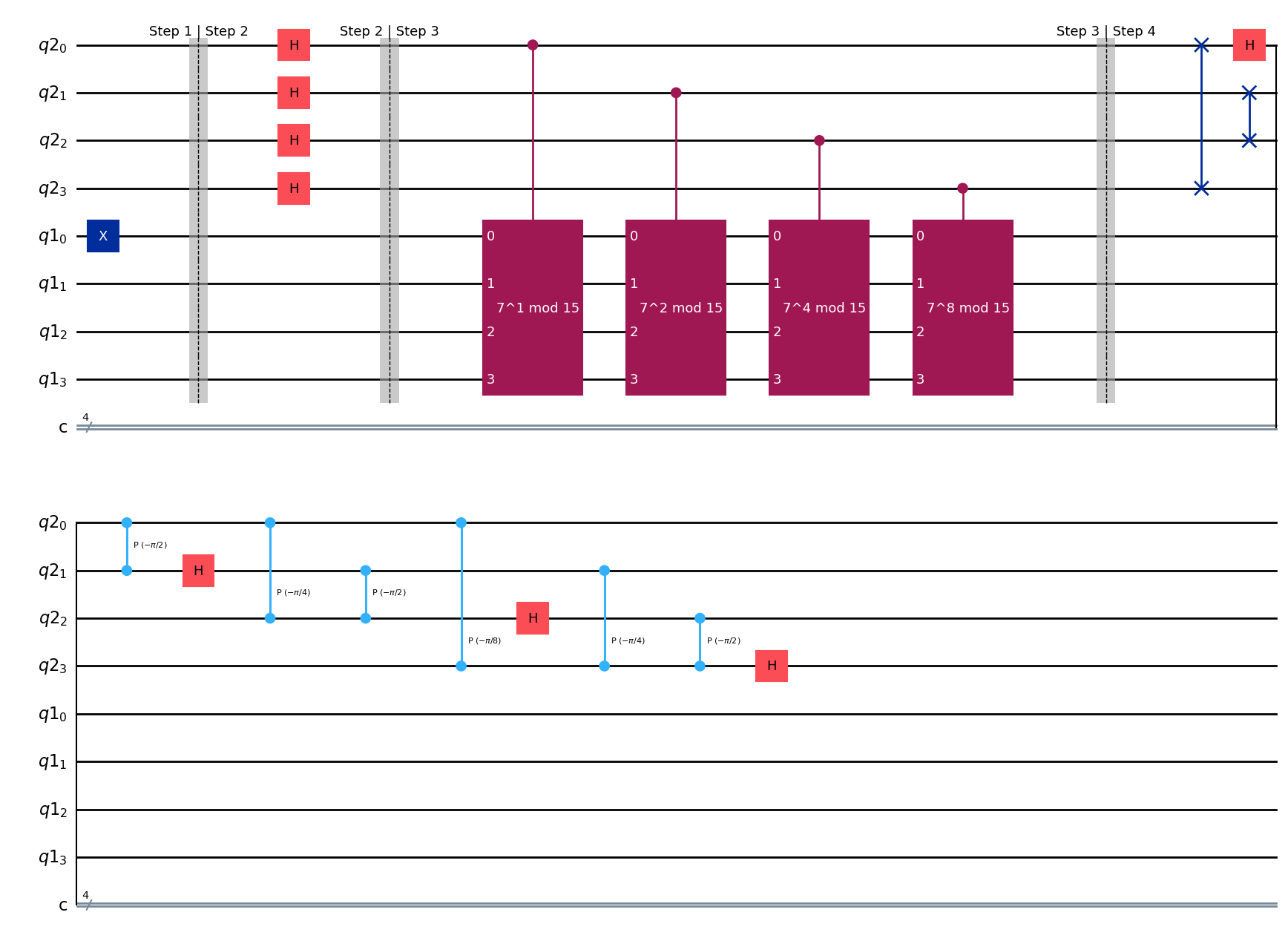
State after Step 3

\[\begin{align*} |\psi_3\rangle & = (U_{7^8 mod 15}^3)(U_{7^4 mod 15}^2)(U_{7^2 mod 15}^1)(U_{7^1 mod 15}^0)|\psi_2\rangle \tag{definition} \\ & = (U_{7^8 mod 15}^3)(U_{7^4 mod 15}^2)(U_{7^2 mod 15}^1)(U_{7^1 mod 15}^0)|0001++++\rangle \tag{definition $|\psi_2\rangle$} \\ & = \frac{1}{\sqrt{2^1}}(U_{7^8 mod 15}^3)(U_{7^4 mod 15}^2)(U_{7^2 mod 15}^1)(|0001+++\rangle \otimes (|0\rangle + e^{2\pi i j/8}|1\rangle)) \tag{Apply U} \\ & = \frac{1}{\sqrt{2^2}}(U_{7^8 mod 15}^3)(U_{7^4 mod 15}^2)(|0001++\rangle (|0\rangle + e^{2\pi i 2j/8}|1\rangle) \otimes (|0\rangle + e^{2\pi i j/8}|1\rangle)) \tag{Apply U} \\ & = \frac{1}{\sqrt{2^3}}(U_{7^8 mod 15}^3)(|0001+\rangle (|0\rangle + e^{2\pi i 4j/8}|1\rangle) \otimes (|0\rangle + e^{2\pi i 2j/8}|1\rangle) \otimes (|0\rangle + e^{2\pi i j/8}|1\rangle)) \tag{Apply U} \\ & = \frac{1}{\sqrt{2^4}}(|0001+\rangle (|0\rangle + e^{2\pi i 8j/8}|1\rangle) \otimes (|0\rangle + e^{2\pi i 4j/8}|1\rangle) \otimes (|0\rangle + e^{2\pi i 2j/8}|1\rangle) \otimes (|0\rangle + e^{2\pi i j/8}|1\rangle)) \tag{Apply U} \\ & = \frac{1}{\sqrt{2^4}}(|0001\rangle (|0\rangle + e^{2\pi i 0.j_3 j_2 j_1 j_0}|1\rangle) \otimes (|0\rangle + e^{2\pi i 0.j_2 j_1 j_0}|1\rangle) \otimes (|0\rangle + e^{2\pi i 0.j_1 j_0}|1\rangle) \otimes (|0\rangle + e^{2\pi i 0.j_0}|1\rangle)) \tag{express j in binary} \\ & = |0001\rangle \otimes F_4|j_3 j_2 j_1 j_0\rangle \tag{QFT binary expansion} \end{align*}\]

Step 4

Apply the inverse QFT to the first register.

Inverse QFT

As a reminder, every quantum operator is invertible. Consequently, we can invert the QFT, resulting in the inverse QFT. We can construct the inverse QFT by applying the inverse of each gate in the QFT in reverse order.

def qft_dagger(qc: QuantumCircuit, n: int) -> None:
    # Swap for little endian
    for qubit in range(n//2):
        qc.swap(qubit, n-qubit-1)
    for j in range(n):
        # Inverse of controlled rotation is inverse rotation
        for m in range(j):
            qc.cp(-np.pi/float(2**(j-m)), m, j)
        # Hadamard is own inverse
        qc.h(j)

# Step 4: Perform inverse QFT
qc.barrier(label="Step 3 | Step 4")
qft_dagger(qc, 4)
qc.draw(output="mpl", style="iqp")

State after Step 4

\[\begin{align*} |\psi_4\rangle & = (I \otimes F_4^{-1}) |\psi_3\rangle \tag{definition} \\ & = (I \otimes F_4^{-1})(|0001\rangle \otimes F_4|j_3 j_2 j_1 j_0\rangle) \tag{definition $|\psi_3\rangle$} \\ & = |0001\rangle \otimes |j_3 j_2 j_1 j_0\rangle \tag{Inverse QFT} \end{align*}\]

Step 5

Measure the first register.

# Step 5: Measure first register
qc.barrier(label="Step 4 | Step 5")
for n in range(n_count):
    qc.measure(n, n)
qc.draw(output="mpl", style="iqp")

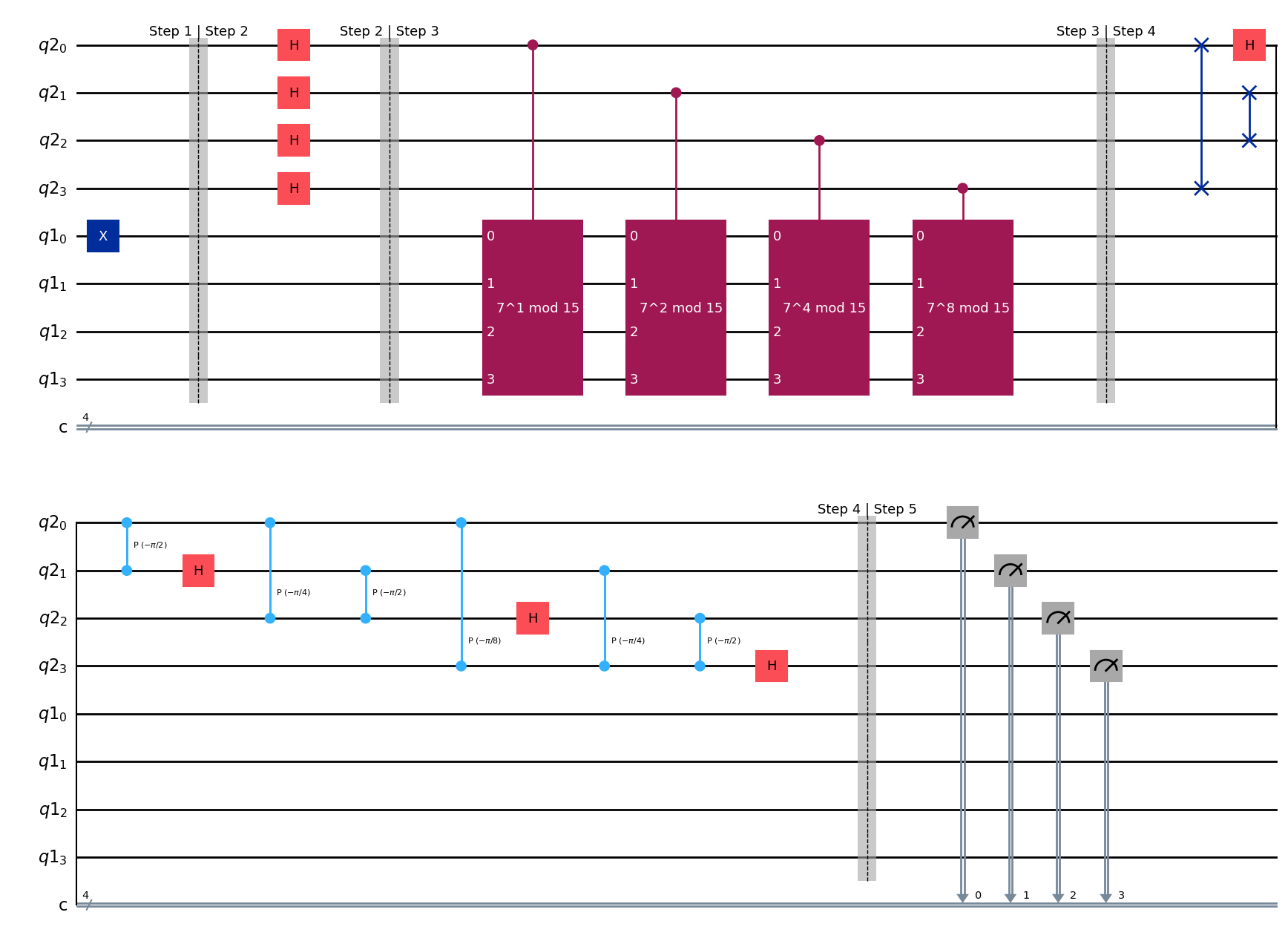
State after Step 5

We have \(|j_3 j_2 j_1 j_0\rangle\). Measurement will produce a multiple of \(j_3 j_2 j_1 j_0\)

t_qpe = transpile(qc, sim)
results = sim.run(t_qpe, shots=2048).result()
counts = results.get_counts()
plot_histogram(counts)

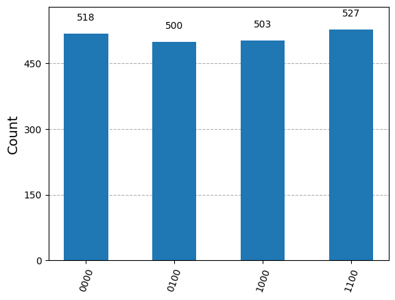
Interpreting the results

1. The order of \(7^x \, (\text{mod} \, 15)\) is \(4\).

2. So our answers should all be multiples of \(4\).

def display_counts(counts):
    rows, measured_phases = [], []
    for output in counts:
        n_count = len(output)
        decimal = int(output, 2)  # Convert (base 2) string to decimal
        phase = decimal/(2**n_count)  # Find corresponding eigenvalue
        measured_phases.append(phase)
        # Add these values to the rows in our table:
        rows.append([f"{output}(bin) = {decimal:>3}(dec)", 
                     f"{decimal}/{2**n_count} = {phase:.2f}"])
    # Print the rows in a table
    headers=["Register Output", "Phase"]
    df = pd.DataFrame(rows, columns=headers)
    return df

display_counts(counts)

	Register Output	Phase
0	0000(bin) = 0(dec)	0/16 = 0.00
1	0100(bin) = 4(dec)	4/16 = 0.25
2	1000(bin) = 8(dec)	8/16 = 0.50
3	1100(bin) = 12(dec)	12/16 = 0.75

Putting it Together

We gather all the steps together now.

def qpe(f_qc_U: Callable, n_count: int) -> QuantumCircuit:
    # Create and set up circuit
    reg1_size = f_qc_U(0).num_qubits
    qc = QuantumCircuit(n_count+reg1_size, n_count)

    # Step 1: Prepare our eigenstate |1>:
    qc.x(n_count)
    
    # Step 2: Apply H-Gates to counting qubits.
    qc.barrier(label="Step 1 | Step 2")
    for qubit in range(n_count):
        qc.h(qubit)
    
    # Step 3: Do the controlled-U operations:
    qc.barrier(label="Step 2 | Step 3")
    for q in range(n_count):
        qc_cU = f_qc_U(2**q).control() # amod15(a, 2**q).control()
        qc.append(qc_cU, [q] + [n_count+i for i in range(reg1_size)])
    
    # Step 4: Perform inverse QFT
    qc.barrier(label="Step 3 | Step 4")
    qft_dagger(qc, 4)
    
    # Step 5: Measure first register
    qc.barrier(label="Step 4 | Step 5")
    for n in range(n_count):
        qc.measure(n, n)
    return qc

qc_qpe = qpe(lambda q: amod15(7, q), 4)
qc_qpe.draw(output="mpl", style="iqp")

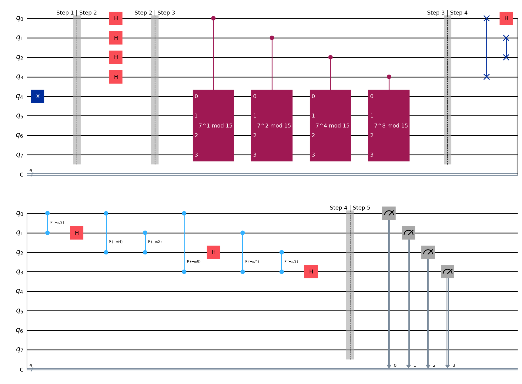
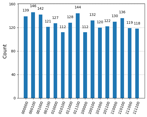
qc_qpe = qpe(lambda q: amod15(7, q), 6)
t_qpe = transpile(qc_qpe, sim)
results = sim.run(t_qpe, shots=2048).result()
counts = results.get_counts()
plot_histogram(counts) # note how the last 2 bits are 00

display_counts(counts)

	Register Output	Phase
0	111000(bin) = 56(dec)	56/64 = 0.88
1	001000(bin) = 8(dec)	8/64 = 0.12
2	001100(bin) = 12(dec)	12/64 = 0.19
3	110100(bin) = 52(dec)	52/64 = 0.81
4	100000(bin) = 32(dec)	32/64 = 0.50
5	110000(bin) = 48(dec)	48/64 = 0.75
6	011000(bin) = 24(dec)	24/64 = 0.38
7	101000(bin) = 40(dec)	40/64 = 0.62
8	111100(bin) = 60(dec)	60/64 = 0.94
9	000000(bin) = 0(dec)	0/64 = 0.00
10	010000(bin) = 16(dec)	16/64 = 0.25
11	100100(bin) = 36(dec)	36/64 = 0.56
12	010100(bin) = 20(dec)	20/64 = 0.31
13	011100(bin) = 28(dec)	28/64 = 0.44
14	000100(bin) = 4(dec)	4/64 = 0.06
15	101100(bin) = 44(dec)	44/64 = 0.69

Summary

1. We have introduced the QPE algorithm.