import numpy as np
import matplotlib.pyplot as plt

from qiskit import QuantumCircuit, QuantumRegister
from qiskit_aer import AerSimulator
from qiskit.quantum_info import Statevector, Operator
from qiskit.visualization import plot_histogram, plot_bloch_multivector
sim = AerSimulator()

from util import zero, one, H, X

Foundations II: Quantum Circuits for Multi-Qubit Systems

We will introduce quantum circuits that act on multi-qubit systems in this notebook. Multi-qubit circuits enable us to entangle qubits and harness the power of quantum computation.

References

1. Introduction to Classical and Quantum Computing: Chapter 4

Multi-Qubit Gates

The building blocks of quantum circuits that operate on multi-qubit systems are multi-qubit gates. A quantum gate \(G\) that acts on two qubits can be represented as a \(4 \times 4\) unitary matrix, i.e., \(G \in \mathcal{U}(4)\). We’ll start with a SWAP gate.

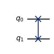
Swap Gate

The SWAP gate swaps two qubits as below

\[ SWAP|q_2 q_1\rangle = |q_1 q_2\rangle \,. \]

qc_swap = QuantumCircuit(2)
qc_swap.swap(0, 1)
qc_swap.draw(output="mpl", style="iqp")

Unitary Matrix for Swap Gate

Like single qubit gates, every two qubit gate also has a corresponding unitary matrix. In the case of a two qubit gate, we have a \(4 \times 4\) unitary matrix. The unitary matrix for a SAWP gate is given below.

SWAP = Operator(qc_swap)
SWAP.draw("latex")

\[\begin{split}\begin{bmatrix} 1 & 0 & 0 & 0 \\ 0 & 0 & 1 & 0 \\ 0 & 1 & 0 & 0 \\ 0 & 0 & 0 & 1 \\ \end{bmatrix} \end{split}\]

# Swapping |10> to |01>
np.allclose((zero ^ one).evolve(SWAP), one ^ zero)

True

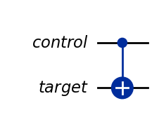
CNOT Gate

1. The cnot gate is a two qubit gate with a control qubit and a target qubit.

2. If the control qubit is set, it flips the target qubit.

3. Otherwise, it does nothing.

control = QuantumRegister(1, "control")
target = QuantumRegister(1, "target")
qc_cnot = QuantumCircuit(control, target)
qc_cnot.cx(0, 1)  # 0 is control, 1 is target
qc_cnot.draw(output="mpl", style="iqp")

The unitary matrix for a CNOT gate is given below.

CNOT = Operator(qc_cnot)
CNOT.draw("latex")

\[\begin{split}\begin{bmatrix} 1 & 0 & 0 & 0 \\ 0 & 0 & 0 & 1 \\ 0 & 0 & 1 & 0 \\ 0 & 1 & 0 & 0 \\ \end{bmatrix} \end{split}\]

# |00> -> |00> (reminder, little endian)
print((zero ^ zero).evolve(Operator(qc_cnot)))
# |01> -> |01> (reminder, little endian)
print((one ^ zero).evolve(Operator(qc_cnot)))
# |10> -> |11> (reminder, little endian)
print((zero ^ one).evolve(Operator(qc_cnot)))
# |11> -> |10> (reminder, little endian)
print((one ^ one).evolve(Operator(qc_cnot)))

Statevector([1.+0.j, 0.+0.j, 0.+0.j, 0.+0.j],
            dims=(2, 2))
Statevector([0.+0.j, 0.+0.j, 1.+0.j, 0.+0.j],
            dims=(2, 2))
Statevector([0.+0.j, 0.+0.j, 0.+0.j, 1.+0.j],
            dims=(2, 2))
Statevector([0.+0.j, 1.+0.j, 0.+0.j, 0.+0.j],
            dims=(2, 2))

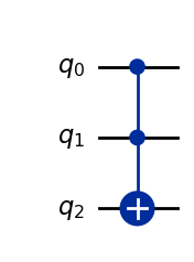
Toffoli gate

The Toffoli gate, notated CCX, is an example of a three qubit gate. A quantum gate \(G\) that acts on three qubits can be represented as a \(8 \times 8\) unitary matrix, i.e., \(G \in \mathcal{U}(8)\).

qc_ccx = QuantumCircuit(3)
qc_ccx.ccx(0, 1, 2)
qc_ccx.draw(output="mpl", style="iqp")

Operator(qc_ccx).draw("latex")   # another advantage of quantum circuits ...

\[\begin{split}\begin{bmatrix} 1 & 0 & 0 & 0 & 0 & 0 & 0 & 0 \\ 0 & 1 & 0 & 0 & 0 & 0 & 0 & 0 \\ 0 & 0 & 1 & 0 & 0 & 0 & 0 & 0 \\ 0 & 0 & 0 & 0 & 0 & 0 & 0 & 1 \\ 0 & 0 & 0 & 0 & 1 & 0 & 0 & 0 \\ 0 & 0 & 0 & 0 & 0 & 1 & 0 & 0 \\ 0 & 0 & 0 & 0 & 0 & 0 & 1 & 0 \\ 0 & 0 & 0 & 1 & 0 & 0 & 0 & 0 \\ \end{bmatrix} \end{split}\]

Multi-Qubit Circuits

Similarly to single-qubit circuits, we can construct multi-qubit circuits out of single-qubit gates and multi-qubit gates. Multi-qubit gates can be sequenced and are reversible.

Property 1: Gates in parallel correspond to tensor product

In a multi-qubit system, we can apply gates to different subset of qubits, i.e., in parallel. Below, we give an example where we apply an \(H\) gate to \(|q_0\rangle\) and a \(X\) gate to \(|q_1\rangle\).

# 2-qubit system
qc_xh = QuantumCircuit(2)
qc_xh.h(0)
qc_xh.x(1)
qc_xh.draw(output="mpl", style="iqp")

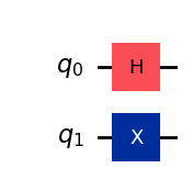
The unitary matrix that corresponds to the two qubit gate that acts on \(|q_1 q_0\rangle\) is given by \(X \otimes H\) where \(\otimes\) is the tensor product.

Aside: Tensor Product on Matrices

Let

\[\begin{split} A = \begin{pmatrix} a_{11} & \dots & a_{1n} \\ \vdots & \ddots & \vdots \\ a_{n1} & \dots & a_{nn} \\ \end{pmatrix} \end{split}\]

and

\[ B^{(m \times m)} \,. \]

Then

\[\begin{split} A \otimes B = \begin{pmatrix} a_{11} B & \dots & a_{1n} B \\ \vdots & \ddots & \vdots \\ a_{1n} B & \dots & a_{nn} B \\ \end{pmatrix} \,. \end{split}\]

Example worked put

\[\begin{align*} X \otimes H & = \begin{pmatrix} 0 & 1 \\ 1 & 0 \\ \end{pmatrix} \otimes \begin{pmatrix} 1/\sqrt{2} & 1/\sqrt{2} \\ 1/\sqrt{2} & -1/\sqrt{2} \\ \end{pmatrix} \\ & = \begin{pmatrix} 0 & 0 & 1/\sqrt{2} & 1/\sqrt{2} \\ 0 & 0 & 1/\sqrt{2} & -1/\sqrt{2} \\ 1/\sqrt{2} & 1/\sqrt{2} & 0 & 0 \\ 1/\sqrt{2} & -1/\sqrt{2} & 0 & 0 \\ \end{pmatrix} \end{align*}\]

# Checking out our worked out example
Operator(qc_xh).draw("latex")

\[\begin{split}\begin{bmatrix} 0 & 0 & \frac{\sqrt{2}}{2} & \frac{\sqrt{2}}{2} \\ 0 & 0 & \frac{\sqrt{2}}{2} & - \frac{\sqrt{2}}{2} \\ \frac{\sqrt{2}}{2} & \frac{\sqrt{2}}{2} & 0 & 0 \\ \frac{\sqrt{2}}{2} & - \frac{\sqrt{2}}{2} & 0 & 0 \\ \end{bmatrix} \end{split}\]

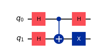
Property 2: Sequencing corresponds to matrix multiplication

We can also sequence multi-qubit gates as we did with single-qubit gates.

qc = QuantumCircuit(2)
qc.h(0)
qc.x(1)
qc.cx(0, 1)
qc.h(1)
qc.h(0)
qc.draw(output="mpl", style="iqp")

In matrix notation (again remembering little endian) … $\( qc = (H \otimes H) \, \text{CNOT} \, (X \otimes H) \)$

op = (X.tensor(H)).compose(CNOT).compose(H.tensor(H))
op.draw("latex")

\[\begin{split}\begin{bmatrix} \frac{\sqrt{2}}{2} & 0 & \frac{\sqrt{2}}{2} & 0 \\ 0 & \frac{\sqrt{2}}{2} & 0 & \frac{\sqrt{2}}{2} \\ 0 & - \frac{\sqrt{2}}{2} & 0 & \frac{\sqrt{2}}{2} \\ - \frac{\sqrt{2}}{2} & 0 & \frac{\sqrt{2}}{2} & 0 \\ \end{bmatrix} \end{split}\]

np.allclose(Operator(qc), op)

True

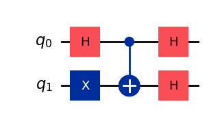
Property 3: Reversability

1. Recall that every unitary \(U\) has a conjugate transpose \(U^\dagger\) such that \(UU^\dagger = I\).

2. Fact: \((ABC)^\dagger = C^\dagger B^\dagger A^\dagger\).

Thus $\( ((X \otimes H) \, \text{CNOT} \, (H \otimes H))^\dagger = (H \otimes H)^\dagger \, \text{CNOT}^\dagger \, (X \otimes H)^\dagger \)$

# cnot is its own inverse
CNOT.compose(CNOT).draw("latex")

\[\begin{split}\begin{bmatrix} 1 & 0 & 0 & 0 \\ 0 & 1 & 0 & 0 \\ 0 & 0 & 1 & 0 \\ 0 & 0 & 0 & 1 \\ \end{bmatrix} \end{split}\]

qc_rev = QuantumCircuit(2)
qc_rev.h(1)
qc_rev.h(0)
qc_rev.cx(0, 1)
qc_rev.h(0)
qc_rev.x(1)
qc_rev.draw(output="mpl", style="iqp")

# Should be close to identity
np.allclose(Operator(qc_rev).compose(Operator(qc)), np.eye(4))

True

Entanglement

Multi-qubit circuits enable us to construct entangled qubits which we can harness to leverage the exponential representational capacity of a a system of \(n\)-qubits without incurring an exponential number of operations. Before we give an example of how to entangle qubits with a multi-qubit circuit, we’ll discuss the situation where two qubits are not entangled in a multi-qubit system.

Non-entangled Computations

As a reminder, two qubits are said to be entangled if they cannot be written as the tensor product of two single qubit systems. A multi-qubit circuit that acts on unentangled qubits can be thus be applied in parallel.

Example

Suppose we run two single qubit systems that are run in parallel.

# 2 circuits in parallel
qc_h = QuantumCircuit(QuantumRegister(1, "q_0")); qc_h.h(0)
qc_x = QuantumCircuit(QuantumRegister(1, "q_1")); qc_x.x(0);

# Top part
qc_h.draw(output="mpl", style="iqp")

# Bottom part
qc_x.draw(output="mpl", style="iqp")

This is equivalent to this circuit from before.

qc_xh.draw(output="mpl", style="iqp")

# Checking that the tensor product of the circuits gives the original multi-qubit circuit
np.allclose(X.tensor(H), Operator(qc))

False

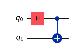
Constructing the Bell State: An Entangled State

Recall the Bell state

\[ \frac{1}{\sqrt{2}}|00\rangle + \frac{1}{\sqrt{2}}|11\rangle \]

was an entangled state. We can use a multi-qubit circuit to construct the Bell state, and thus, entangle two qubits.

qc_bell = QuantumCircuit(2)
qc_bell.h(0)
qc_bell.cx(0, 1)
qc_bell.draw(output="mpl", style="iqp")

(zero ^ zero).evolve(Operator(qc_bell)).draw("latex")

\[\frac{\sqrt{2}}{2} |00\rangle+\frac{\sqrt{2}}{2} |11\rangle\]

Summary

1. We introduced multi-qubit gates, including the CNOT gate.

2. We saw that a multi-qubit circuits can be used to entangle qubits.