from typing import *
import time
import random
import numpy as np
import matplotlib.pyplot as plt

from qiskit_aer import AerSimulator
from qiskit.quantum_info import Statevector, Operator
from qiskit.visualization import plot_histogram, plot_bloch_multivector
from qiskit import QuantumCircuit, QuantumRegister, ClassicalRegister
sim = AerSimulator()

from util import zero, one, enum_bits

QC: Simon’s Algorithm

Simon’s Algorithm was the first quantum algorithm to demonstrate exponential speedup compared to classical probabilistic algorithm. Thus, it improves upon Deutch-Jozsa and gives hope that there are a class of problems that can be solved with a quantum computer that cannot be solved with a classical computer.

References

1. Qiskit notebook on Simon’s algorithm

Problem Formulation

Simon’s algorithm solves the problem of determining whether a function is one-to-one or two-to-one. Similar to Deutsch-Jozsa, Simon’s algorithm solves a somewhat contrived problem whose main utility is in showing that it is possible for a quantum algorithm to achieve exponential speedup compared to a classical algorithm.

One-to-one function

A function \(f: \{0, 1\}^n \rightarrow \{0, 1\}^n\) is one-to-one if

\[ f(x) = f(y) \]

iff \(x = y\), i.e., it maps unique bitstrings to unique bitstrings.

# one-to-one
def neg_all(x: list[bool]) -> list[bool]:
    return [not b for b in x]

print(neg_all([False, False]))
print(neg_all([False, True]))
print(neg_all([True, False]))
print(neg_all([True, True]))

[True, True]
[True, False]
[False, True]
[False, False]

# not one-to-one
def f(x: list[bool]) -> list[bool]:
    return [x[len(x)-1]] + [x[i] and x[i+1] for i in range(len(x)-1)]

print(f([False, False])) # <- non-unique
print(f([False, True]))
print(f([True, False]))  # <- non-unique
print(f([True, True]))

[False, False]
[True, False]
[False, False]
[True, True]

Two-to-one function

A function \(f: \{0, 1\}^n \rightarrow \{0, 1\}^n\) is two-to-one if for every unique output \(z\),

\[ z = f(x) = f(y) \]

for exactly two \(x \neq y\), i.e., it maps each pair of unique bit-strings to the same output.

Equivalent formulation

1. Equivalently, let \(b \in \{0, 1\}^n \neq 0\) be a bit string. Then \(f\) is two-to-one if \(f(x) = f(y)\) iff \(y = x \oplus b\).

2. Note that \(b = 0\dots0\) corresponds to the case that f is a one-to-one function.

def mk_two2one_nbit(n) -> list[bool]:
    b = [True] + [random.choice([True, False]) for i in range(n-1)]
    xs = enum_bits(len(b))
    out = enum_bits(len(b)); random.shuffle(out); i = 0
    mapping = {}; seen = set()
    for x in xs:
        y = [c != d for c, d in zip(x, b)]
        sx = str(x); sy = str(y);
        if sx in seen or sy in seen:
            continue
        mapping[sx] = out[i]; mapping[sy] = out[i]; i += 1
        seen.add(sx); seen.add(sy)
    
    return lambda x: mapping[str(x)]

g2 = mk_two2one_nbit(2)
print(g2([False, False]))
print(g2([False, True]))
print(g2([True, False]))
print(g2([True, True]))

[False, True]
[True, True]
[True, True]
[False, True]

g3 = mk_two2one_nbit(3)
for b in enum_bits(3):
    print(g3(b))

[True, True, True]
[True, True, True]
[False, True, True]
[False, True, True]
[True, True, False]
[True, True, False]
[True, False, False]
[True, False, False]

Simon’s Problem Formulation

Simon’s problem is: given a function on bitstrings \(f : \{0, 1\}^n \rightarrow \{0, 1\}^n\) that is either

1. a one-to-one function or

2. a two-to-one function,

determine whether it is a one-to-one function or a two-to-one function. Equivalently, given a hidden bit string \(b\), determine if \(b\) is all 0s or not.

Classical Solution

Intuitively, the simplest thing we can do is to check every input and see if we get a one-to-one function or a two-to-one function. We actually “only” need to check one more than half of the inputs since we’re dealing with two-to-one functions.

def solve_simons(nbits: int, f: Callable[list[bool], list[bool]]) -> str:
    seen = set()
    inputs = enum_bits(nbits)
    count = 0
    for b in inputs:
        # We only need to check half the inputs
        if count >= len(inputs)/2 + 1:
            break
        count += 1
        
        # Keep track of what we have seen
        y = str(f(b))
        if y in seen:
            return "two-to-one"
        seen.add(y)
    return "one-to-one"

solve_simons(3, neg_all)

'one-to-one'

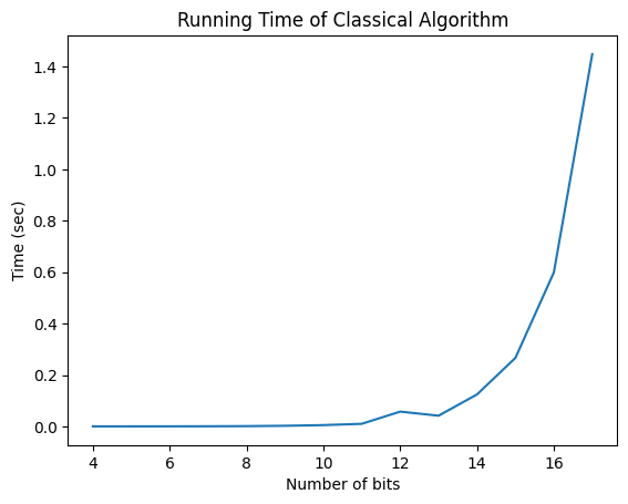
ns = range(4, 18)
times = []
for n in ns:
    start = time.time()
    gn = mk_two2one_nbit(n)
    solve_simons(n, gn)
    times += [time.time() - start]
plt.plot(ns, times)
plt.xlabel('Number of bits'); plt.ylabel('Time (sec)'); plt.title('Running Time of Classical Algorithm')

Text(0.5, 1.0, 'Running Time of Classical Algorithm')

Aside: Probabilistic Solution to Simon’s Problem

Unlike the Deutsch-Jozsa problem, it is still hard for us to get a speedup, even if we allowed for some error. Intuitively, we still need to check half the bit-strings (in the worst case since the two-to-one can be adversarially constructed), which would still take exponential time.

Quantum Solution

In this section, we’ll walkthrough Simon’s algorithm. Simon’s algorithm provides an efficient solution to distinguishing between two-to-one or one-to-one functions.

Walkthrough

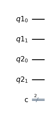
We’ll use a two qubit example. It will be helpful to separate the initial state

\[ |\psi_0 \rangle = |0\rangle^{\otimes n} \otimes |0\rangle^{\otimes n} \]

into two parts.

b = "11"
n = len(b)
part1 = QuantumRegister(n, "q1")
part2 = QuantumRegister(n, "q2")
output = ClassicalRegister(n, "c")
simon_circuit = QuantumCircuit(part1, part2, output)
simon_circuit.draw(output="mpl", style="iqp")

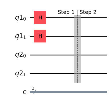
Step 1: Put first n qubits in superposition

Our first step is to the first \(n\) qubits in superposition. Towards this end, we apply \(H^{\otimes n} = \frac{1}{\sqrt{2^n}} \sum_{x \in \{0, 1\}^n} \sum_{y \in \{0, 1\}^n}(-1)^{x \cdot y} |x\rangle\langle y|\) to the first \(n\) qubits.

# Step 1: Apply Hadamard gates to first n qubits
simon_circuit.h(range(n))    
simon_circuit.barrier(label="Step 1 | Step 2")
simon_circuit.draw(output="mpl", style="iqp")

State after step 1

After we apply step 1, we have the following quantum state

\[\begin{align*} |\psi_1 \rangle & = (I^{\otimes n} \otimes H^{\otimes n}) |\psi_0 \rangle \tag{Step 2} \\ & = |0\rangle^{\otimes n} \otimes \left( \frac{1}{\sqrt{2^n}} \sum_{x \in \{0, 1\}^n} \sum_{y \in \{0, 1\}^n}(-1)^{x \cdot y} |x\rangle\langle y||0\rangle^{\otimes n} \right) \tag{definition $H^{\otimes n}$ and linearity} \\ & = |0\rangle^{\otimes n} \otimes \frac{1}{\sqrt{2^n}} \sum_{x \in \{0, 1\}^n} (-1)^{x \cdot |0\rangle^{\otimes n}}|x\rangle \tag{non-zero when $y = |0\rangle^{\otimes n}$} \\ & = |0\rangle^{\otimes n} \otimes \frac{1}{\sqrt{2^n}} \sum_{x \in \{0, 1\}^n} |x\rangle \tag{dot product is $0$} \\ & = \frac{1}{\sqrt{2^n}} \sum_{x \in \{0, 1\}^n} |0^{\otimes n}, x\rangle \tag{rearrange} \end{align*}\]

Step 2: Apply Oracle

Apply the oracle

\[ U_f|y, x\rangle = U_f|y \oplus f(x), x\rangle \,. \]

# Source: https://github.com/qiskit-community/qiskit-textbook/blob/589c64d66c8743c123c9704d9b66cda4d476dbff/qiskit-textbook-src/qiskit_textbook/tools/__init__.py
def simon_oracle(b):
    """returns a Simon oracle for bitstring b"""
    b = b[::-1] # reverse b for easy iteration
    n = len(b)
    qc = QuantumCircuit(n*2)
    # Do copy; |x>|0> -> |x>|x>
    for q in range(n):
        qc.cx(q, q+n)
    if '1' not in b: 
        return qc  # 1:1 mapping, so just exit
    i = b.find('1') # index of first non-zero bit in b
    # Do |x> -> |s.x> on condition that q_i is 1
    for q in range(n):
        if b[q] == '1':
            qc.cx(i, (q)+n)
    return qc 

oracle = simon_oracle(b)

# Step 2: Query Oracle
simon_circuit = simon_circuit.compose(oracle)
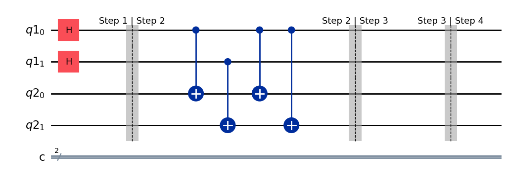
simon_circuit.barrier(label="Step 2 | Step 3")
simon_circuit.draw(output="mpl", style="iqp")

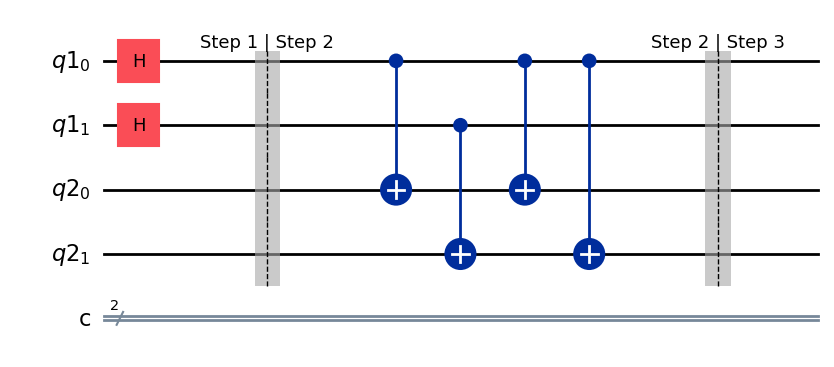
After step 2

After we apply the oracle, we have the following quantum state

\[\begin{align*} |\psi_2\rangle & = H^{\otimes n} |\psi_1\rangle \tag{Step 3} \\ & = \frac{1}{\sqrt{2^n}} \sum_{x \in \{0, 1\}^n} U_f |0^{\otimes n}, x\rangle \tag{definition $H^{\otimes n}$ and linearity} \\ & = \frac{1}{\sqrt{2^n}} \sum_{x \in \{0, 1\}^n} |0^{\otimes n} \oplus f(x), x\rangle \tag{apply oracle} \\ & = \frac{1}{\sqrt{2^n}} \sum_{x \in \{0, 1\}^n} |f(x), x\rangle \tag{property of xor $\oplus$} \,. \end{align*}\]

Observe that we have now encoded the result of the oracle as part of a computational basis vector.

Step 3: Measure second n qubits

Measure the second half of \(|\psi_2\rangle\) to obtain \(f(x)\).

# Can only measure at the end in qiskit
simon_circuit.barrier(label="Step 3 | Step 4")
simon_circuit.draw(output="mpl", style="iqp")

After step 3

After measuring the second half of \(|\psi_2\rangle\) to obtain \(f(x)\), this means either \(x\) or \(y = x \oplus b\) could be the corresponding input. Therefore the first half of \(|\psi_2\rangle\) becomes

\[ |\psi_3\rangle = \frac{1}{\sqrt{2}} (|x\rangle + |y\rangle) \]

so that the entire quantum state is

\[ |f(x) \rangle \otimes |\psi_3\rangle \,. \]

Step 4: Prepare for measurement

Apply \(H^{\otimes n} = \frac{1}{\sqrt{2^n}} \sum_{x \in \{0, 1\}^n} \sum_{y \in \{0, 1\}^n}(-1)^{x \cdot y} |x\rangle\langle y|\) to the first \(n\) qubits, i.e., \(|\psi_3\rangle\) to prepare for measurement.

simon_circuit.h(range(n))
simon_circuit.barrier(label="Step 4 | Step 5")
simon_circuit.draw(output="mpl", style="iqp")

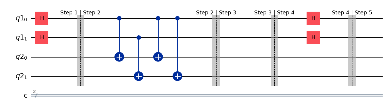
State after step 4

After step 4, we obtain the following quantum state

\[\begin{align*} |\psi_4\rangle & = H^{\otimes n} |\psi_3\rangle \tag{Step 5} \\ & = H^{\otimes n} \frac{1}{\sqrt{2}} (|x\rangle + |y\rangle) \tag{substitute $|\psi_4\rangle$} \\ & = \frac{1}{\sqrt{2^{n+1}}} \sum_{w \in \{0, 1\}^n} \sum_{z \in \{0, 1\}^n}(-1)^{w \cdot z} |w\rangle\langle z|(|x\rangle + |y\rangle) \tag{definition H and linearity} \\ & = \frac{1}{\sqrt{2^{n+1}}} \sum_{w \in \{0, 1\}^n} ((-1)^{w \cdot x} + (-1)^{w \cdot y}) |w\rangle \tag{dot product not zero when z = x or z = y} \,. \end{align*}\]

We have “leaked” the dot product \(w \cdot x\) and \(w \cdot y\) into the phase of \(|\psi_4\rangle\).

Step 5: Measure first n qubits

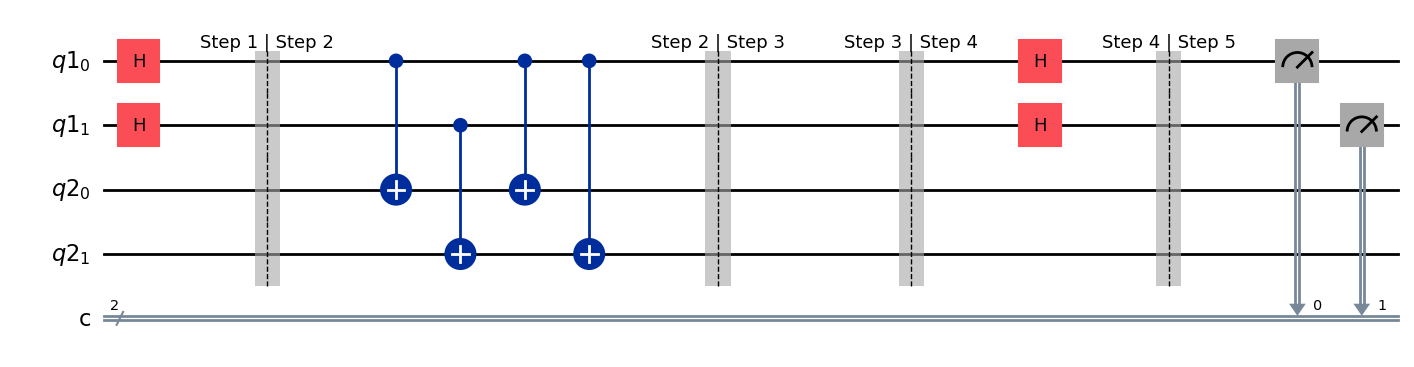
The last step in the algorithm is to measure the first n qubits.

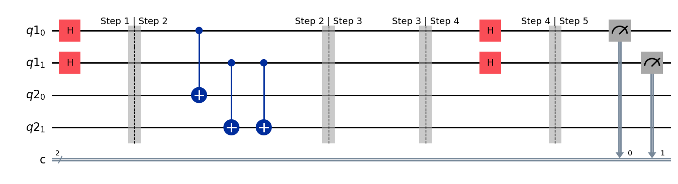
simon_circuit.measure(range(n), range(n))
simon_circuit.draw(output="mpl", style="iqp")

Interpreting the results

Observe:

1. \((-1)^{w \cdot x} = (-1)^{w \cdot y}\): contribution of corresponding \(|a\rangle\)

2. \((-1)^{w \cdot x} \neq (-1)^{w \cdot y}\): no contribution of corresponding \(|w\rangle\)

Consequently, upon a single measurement, we will observe some \(|w\rangle\) s.t. \(w \cdot x = w \cdot y\). This occurs

\[\begin{align*} w \cdot x = a \cdot y & \iff w \cdot x = w \cdot (x \oplus b) \tag{substitute y} \\ & \iff w \cdot x = (w \cdot x) \oplus (w \cdot b) \tag{property of xor $\oplus$} \\ & \iff 0 = w \cdot b \,. \tag{xor both sides by $(w \cdot x)$} \\ \end{align*}\]

Thus with \(\approx n\) queries, we obtain a system of linear equations

\[\begin{align*} w_1 \cdot b & = 0 \tag{measurement 1}\\ \vdots & = 0 \\ w_n \cdot b & = 0 \tag{measurement n}\\ \end{align*}\]

This can be solved in \(O(n^3)\) time.

# Calculate the dot product of the results
def bdotz(b, z):
    # Source: https://qiskit.org/textbook/ch-algorithms/simon.html
    accum = 0
    for i in range(len(b)):
        accum += int(b[i]) * int(z[i])
    return (accum % 2)

results = sim.run(simon_circuit, shots=1024).result()
counts = results.get_counts()
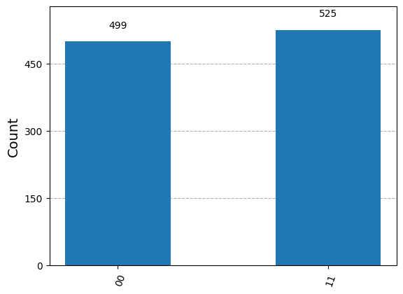
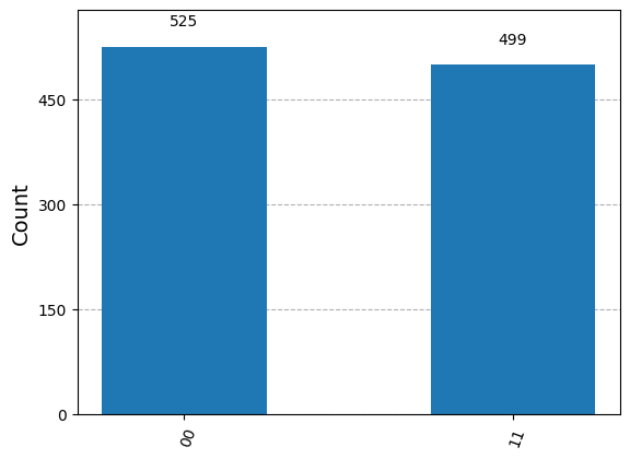
for z in counts:
    print("{}.{} = {} (mod 2)".format(b, z, bdotz(b,z)))
plot_histogram(counts)

11.11 = 0 (mod 2)
11.00 = 0 (mod 2)

Putting it together

We provide the full algorithm below.

def simons(b: str) -> QuantumCircuit:
    n = len(b)
    oracle = simon_oracle(b)
    part1 = QuantumRegister(n, "q1")
    part2 = QuantumRegister(n, "q2")
    output = ClassicalRegister(n, "c")
    simon_circuit = QuantumCircuit(part1, part2, output)

    # Step 1: Apply Hadamard gates to first n qubits
    simon_circuit.h(range(n))    
    simon_circuit.barrier(label="Step 1 | Step 2")

    # Step 2: Query Oracle
    simon_circuit = simon_circuit.compose(oracle)
    simon_circuit.barrier(label="Step 2 | Step 3")

    # Step 3: Can only measure in qiskit at the end, but these results are ignored
    simon_circuit.barrier(label="Step 3 | Step 4")

    # Step 4: Apply Hadamard gates to first n qubits
    simon_circuit.h(range(n))  
    simon_circuit.barrier(label="Step 4 | Step 5")

    # Step 5: Measure first n qubits
    simon_circuit.measure(range(n), range(n))
    
    return simon_circuit

simon_circuit2 = simons("10")
simon_circuit2.draw(output="mpl", style="iqp")

results = sim.run(simon_circuit, shots=1024).result()
counts = results.get_counts()
for z in counts:
    print("{}.{} = {} (mod 2)".format(b, z, bdotz(b,z)))
plot_histogram(counts)

11.11 = 0 (mod 2)
11.00 = 0 (mod 2)

Summary

1. The classical algorithm for solving Simon’s problem requires an exponential number of queries.

2. The quantum algorithm for solving Simon’s problem requires just a single query.

3. Simon’s algorithm is contrived. Nevertheless, it inspired Shor’s algorithm, which is useful.