import math
from typing import *
import numpy as np
import matplotlib.pyplot as plt

from qiskit.quantum_info import Statevector, Operator
from qiskit.visualization import plot_bloch_vector
from qiskit import QuantumCircuit
from qiskit_aer import AerSimulator
sim = AerSimulator()

from util import zero, one, statevector_to_bloch_vector

Shor’s Part 2/5: The Quantum Fourier Transform

The Quantum Fourier Transform (QFT), by analogy with the classical Fourier Transform, represents a quantum state in the “frequency” domain. It is a fundamental building block in Shor’s algorithm where the periodicities in data can be extracted to factor integers efficiently.

References

1. Introduction to Classical and Quantum Computing, Chapter 7.7.3

2. https://qiskit.org/textbook/ch-algorithms/quantum-fourier-transform.html

3. Introduction to Quantum Information Science: Lectures 19 and 20 by Scott Aaronson

4. Quantum Computation and Quantum Information: Chapter 5, Nielsen and Chuang

Definition

The Quantum Fourier Transform (QFT) over \(t\) qubits (\(T = 2^t\)) is defined as the \(T \times T\) matrix \(F_T\) whose \(j\)-th and \(k\)-th entry is

\[\begin{align*} (F_T)_{j, k} & = \omega^{j k}_T \end{align*}\]

where

\[ \omega_{T}^{jk} = e^{2\pi i \frac{jk}{T}} \]

is a root of unity.

def root_of_unity(j: int, k: int, T: int) -> np.complex64:
    return np.exp(2 * np.pi * 1j * j * k / T)

def mk_F(T: int) -> Operator:
    return 1/np.sqrt(T) * Operator([[root_of_unity(j, k, T) for j in range(0, T)] for k in range(0, T)])

Aside: Roots of unity

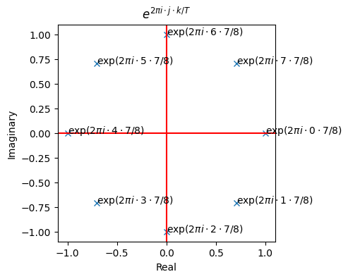
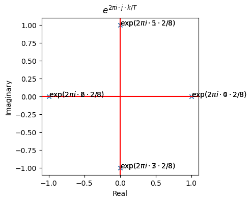
We can visualize a root of unity on the unit circle.

def plot_roots_of_unity(k: int, T: int) -> None:
    fig = plt.figure(figsize=(4, 4)); ax = fig.add_subplot()
    ax.set_aspect(1.0/ax.get_data_ratio(), adjustable='box')

    # Plot
    jks = [(j, k) for j in range(T)]
    txt = [f"exp(2$\\pi i\\cdot{j}\\cdot{k}/{T})$" for i, (j, k) in enumerate(jks)]
    zs = [np.exp(2*np.pi*j*k/T*1j) for j, k in jks]
    for i, t in enumerate(txt):
        plt.annotate(t, (zs[i].real, zs[i].imag))

    # Plot meta-data
    plt.plot([z.real for z in zs], [z.imag for z in zs], linestyle="none", marker='x')
    plt.axhline(y=0.0, color="r", linestyle="-"); plt.axvline(x=0.0, color="r", linestyle="-")
    plt.xlabel("Real"); plt.ylabel("Imaginary"); plt.title(r"$e^{2 \pi i \cdot j \cdot k/T}$");

# k = 1, so it takes us 8 traverses to reach our starting point
plot_roots_of_unity(1, 8)

# k = 7, so it takes us 8 traverses to reach the starting point
plot_roots_of_unity(7, 8)

# k = 2, so it takes us 4 traverses to reach the starting point
plot_roots_of_unity(2, 8)

Root of Unity Encodes Period Information

For any arbitrary starting point, the number of times needed to cycle back to that point encodes information about the period \(T\). For instance,

• 8 traverses implies either \(k = 1\) or \(k = 7\) and \(T = 8\).

• Similarly, 2 traverses implies either \(k = 2\) and \(T = 8\) or \(k = 6\) and \(T = 8\).

Thus a root of unity \(\omega_T^{jk}\) encodes the number of times needed to reach the starting point, without needing to know the starting point!

Examples

To unpack the formal definition of a QFT, we’ll give a few examples now.

Example: QFT on 1 Qubit

Unpacking the definition for \(T = 2\), we obtain

\[\begin{align*} F_2 & = \frac{1}{\sqrt{2}} \begin{pmatrix} \omega_2^{0 \cdot 0} & \omega_2^{1 \cdot 0} \\ \omega_2^{0 \cdot 1} & \omega_2^{1 \cdot 1} \end{pmatrix} \\ & = \frac{1}{\sqrt{2}} \begin{pmatrix} 1 & 1 \\ 1 & -1 \\ \end{pmatrix} \,. \end{align*}\]

This is a Hadamard gate!

F_2 = mk_F(2)
F_2.draw("latex")

\[\begin{split}\begin{bmatrix} \frac{\sqrt{2}}{2} & \frac{\sqrt{2}}{2} \\ \frac{\sqrt{2}}{2} & - \frac{\sqrt{2}}{2} \\ \end{bmatrix} \end{split}\]

\(F_2\) on basis

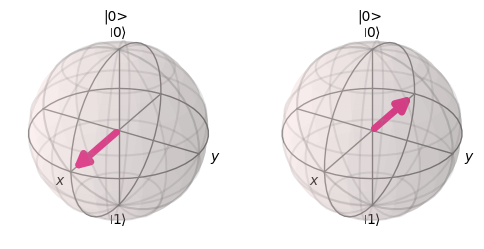
We can visualize the effect of \(F_2\) on the computational basis. In particular, it maps the computational basis into the \(|+\rangle\) and \(|-\rangle\) basis.

fig = plt.figure(figsize = [6, 9])
ax1 = fig.add_subplot(1, 2, 1, projection="3d")
ax2 = fig.add_subplot(1, 2, 2, projection="3d")

# Using global phase
plot_bloch_vector(statevector_to_bloch_vector(zero.evolve(F_2)), ax=ax1, title="|0>")
plot_bloch_vector(statevector_to_bloch_vector(one.evolve(F_2)), ax=ax2, title="|0>")

Example: QFT on 2 Qubits

\[\begin{align*} F_4 & = \frac{1}{2}\begin{pmatrix} \omega_2^{0 \cdot 0} & \omega_2^{1 \cdot 0} & \omega_2^{2 \cdot 0} & \omega_2^{3 \cdot 0} \\ \omega_2^{0 \cdot 1} & \omega_2^{1 \cdot 1} & \omega_2^{2 \cdot 1} & \omega_2^{3 \cdot 1} \\ \omega_2^{0 \cdot 2} & \omega_2^{1 \cdot 2} & \omega_2^{2 \cdot 2} & \omega_2^{3 \cdot 2} \\ \omega_2^{0 \cdot 3} & \omega_2^{1 \cdot 3} & \omega_2^{2 \cdot 3} & \omega_2^{3 \cdot 3} \end{pmatrix} \end{align*}\]

F_4 = mk_F(4)
F_4.draw("latex")

\[\begin{split}\begin{bmatrix} \frac{1}{2} & \frac{1}{2} & \frac{1}{2} & \frac{1}{2} \\ \frac{1}{2} & \frac{i}{2} & - \frac{1}{2} & - \frac{i}{2} \\ \frac{1}{2} & - \frac{1}{2} & \frac{1}{2} & - \frac{1}{2} \\ \frac{1}{2} & - \frac{i}{2} & - \frac{1}{2} & \frac{i}{2} \\ \end{bmatrix} \end{split}\]

\(F_4\) on basis

\(F_4\) performs a similar style of transform on the computational basis to \(F_2\). In particular, it maps the computational basis into superpositions of the computational basis.

(zero^zero).evolve(F_4).draw("latex")

\[\frac{1}{2} |00\rangle+\frac{1}{2} |01\rangle+\frac{1}{2} |10\rangle+\frac{1}{2} |11\rangle\]

(zero^one).evolve(F_4).draw("latex")

\[\frac{1}{2} |00\rangle+\frac{i}{2} |01\rangle- \frac{1}{2} |10\rangle- \frac{i}{2} |11\rangle\]

(one^zero).evolve(F_4).draw("latex")

\[\frac{1}{2} |00\rangle- \frac{1}{2} |01\rangle+\frac{1}{2} |10\rangle- \frac{1}{2} |11\rangle\]

(one^one).evolve(F_4).draw("latex")

\[\frac{1}{2} |00\rangle- \frac{i}{2} |01\rangle- \frac{1}{2} |10\rangle+\frac{i}{2} |11\rangle\]

Example: QFT on 3 Qubits

The QFT for 3 qubits is a \(8 \times 8\) matrix.

mk_F(8).draw("latex")

\[\begin{split}\begin{bmatrix} \frac{\sqrt{2}}{4} & \frac{\sqrt{2}}{4} & \frac{\sqrt{2}}{4} & \frac{\sqrt{2}}{4} & \frac{\sqrt{2}}{4} & \frac{\sqrt{2}}{4} & \frac{\sqrt{2}}{4} & \frac{\sqrt{2}}{4} \\ \frac{\sqrt{2}}{4} & \frac{1}{4} + \frac{i}{4} & \frac{\sqrt{2} i}{4} & - \frac{1}{4} + \frac{i}{4} & - \frac{\sqrt{2}}{4} & - \frac{1}{4} - \frac{i}{4} & - \frac{\sqrt{2} i}{4} & \frac{1}{4} - \frac{i}{4} \\ \frac{\sqrt{2}}{4} & \frac{\sqrt{2} i}{4} & - \frac{\sqrt{2}}{4} & - \frac{\sqrt{2} i}{4} & \frac{\sqrt{2}}{4} & \frac{\sqrt{2} i}{4} & - \frac{\sqrt{2}}{4} & - \frac{\sqrt{2} i}{4} \\ \frac{\sqrt{2}}{4} & - \frac{1}{4} + \frac{i}{4} & - \frac{\sqrt{2} i}{4} & \frac{1}{4} + \frac{i}{4} & - \frac{\sqrt{2}}{4} & \frac{1}{4} - \frac{i}{4} & \frac{\sqrt{2} i}{4} & - \frac{1}{4} - \frac{i}{4} \\ \frac{\sqrt{2}}{4} & - \frac{\sqrt{2}}{4} & \frac{\sqrt{2}}{4} & - \frac{\sqrt{2}}{4} & \frac{\sqrt{2}}{4} & - \frac{\sqrt{2}}{4} & \frac{\sqrt{2}}{4} & - \frac{\sqrt{2}}{4} \\ \frac{\sqrt{2}}{4} & - \frac{1}{4} - \frac{i}{4} & \frac{\sqrt{2} i}{4} & \frac{1}{4} - \frac{i}{4} & - \frac{\sqrt{2}}{4} & \frac{1}{4} + \frac{i}{4} & - \frac{\sqrt{2} i}{4} & - \frac{1}{4} + \frac{i}{4} \\ \frac{\sqrt{2}}{4} & - \frac{\sqrt{2} i}{4} & - \frac{\sqrt{2}}{4} & \frac{\sqrt{2} i}{4} & \frac{\sqrt{2}}{4} & - \frac{\sqrt{2} i}{4} & - \frac{\sqrt{2}}{4} & \frac{\sqrt{2} i}{4} \\ \frac{\sqrt{2}}{4} & \frac{1}{4} - \frac{i}{4} & - \frac{\sqrt{2} i}{4} & - \frac{1}{4} - \frac{i}{4} & - \frac{\sqrt{2}}{4} & - \frac{1}{4} + \frac{i}{4} & \frac{\sqrt{2} i}{4} & \frac{1}{4} + \frac{i}{4} \\ \end{bmatrix} \end{split}\]

QFT Encodes Information in Phase

The QFT transform the computational basis into another basis that encodes information in the global phase. To see this, we can rewrite the \(F_T\) with the following formula

\[ F_{T} = \frac{1}{\sqrt{T}} \sum_{j=0}^{T-1} \sum_{k=0}^{T-1} \omega_{T}^{jk}|\overline{k}\rangle \langle \overline{j}| \]

where \(|\overline{j}\rangle\) is the binary encoding in \(t\) bits of the number \(j\).

Using this alternative characterization of the QFT, we can see that it maps each element in the computational basis into a superposition of computational basis elements offset by a global phase as in

\[\begin{align*} F_T |\overline{l}\rangle & = (\frac{1}{\sqrt{T}} \sum_{j=0}^{T-1} \sum_{k=0}^{T-1} \omega_T^{jk}|\overline{k}\rangle \langle \overline{j}|) |\overline{l}\rangle \tag{definition} \\ & = \frac{1}{\sqrt{T}} \sum_{j=0}^{T-1} \sum_{k=0}^{T-1} \omega_T^{jk}|\overline{k}\rangle \langle \overline{j}| |\overline{l}\rangle) \tag{linearity} \\ & = \frac{1}{\sqrt{T}} \sum_{k=0}^{T-1} \omega_T^{lk}|\overline{k}\rangle \tag{orthogonality} \,. \end{align*}\]

Thus the QFT enables the storage of information in the global phase. To foreshadow what’s to come, quantum phase estimation, will be a procedure used to read out information stored in the phase.

Binary Representation of QFT

Define the notation

\[\begin{align*} 0.j_{t-1} \dots j_0 & = \frac{1}{2^t} (j_{t-1} \dots j_0) \\ & = \frac{j_{t-1}}{2} + \dots + \frac{j_0}{2^{t}} \,. \end{align*}\]

Then we can alternatively write the QFT \(F_T\) as

\[ F_T |j_1 \dots j_t\rangle = \frac{(|0\rangle + e^{2\pi i 0.j_0}|1\rangle)(|0\rangle + e^{2\pi i 0.j_1 j_0}|1\rangle)\dots(|0\rangle + e^{2\pi i 0.j_{t-1} \dots j_0}|1\rangle)}{2^{t/2}} \,. \]

Example: F_2

\[\begin{align*} F_2 |j_1\rangle & = \frac{(|0\rangle + e^{2\pi i 0.j_0}|1\rangle)}{2^{1/2}} \\ & = \frac{(|0\rangle + e^{2\pi i j_0/2}|1\rangle)}{\sqrt{2}} \\ \end{align*}\]

Thus

\[ F_2 |0\rangle = \frac{(|0\rangle + |1\rangle)}{\sqrt{2}} \]

and

\[ F_2 |1\rangle = \frac{(|0\rangle - |1\rangle)}{\sqrt{2}} \,. \]

Example: F_4

\[\begin{align*} F_T |j_1 j_2\rangle & = \frac{(|0\rangle + e^{2\pi i 0.j_0}|1\rangle)(|0\rangle + e^{2\pi i 0.j_1j_0}|1\rangle)}{2^{2/2}} \\ & = \frac{(|0\rangle + e^{2\pi i j_0/2}|1\rangle)(|0\rangle + e^{2\pi i (j_1/2 + j_0/4)}|1\rangle)}{2} \\ & = \frac{|00\rangle + e^{2\pi i (j_1/2 + j_0/4)}|01\rangle + e^{2\pi i j_0/2}|10\rangle + e^{2\pi i (j_1/2 + 3j_0/4)|11\rangle}}{2} \\ \end{align*}\]

Thus 1.

\[ F_T |00\rangle = \frac{|00\rangle + |01\rangle + |10\rangle + |11\rangle}{2} \, \]

\[ F_T |01\rangle = \frac{|00\rangle + i|01\rangle - |10\rangle + i|11\rangle}{2} \, \]

\[ F_T |10\rangle = \frac{|00\rangle - |01\rangle + |10\rangle - |11\rangle}{2} \, \]

and

\[ F_T |11\rangle = \frac{|00\rangle - |01\rangle - |10\rangle + |11\rangle}{2} \,. \]

QFT Circuit

It isn’t obvious that we can construct a circuit that implements the QFT with a polynomial number of gates. Thankfull, we can rely on a recurrence relation to make it possible to construct a QFT in \(O(t^2)\) gates.

Observation 1

Applying H to first qubit produces

\[\begin{align*} (I^{t-1} \otimes H) |j_{t-1} \dots j_0\rangle & = \frac{1}{\sqrt{2}}(|0\rangle + e^{2\pi i 0.j_0}|1\rangle) |j_{t-1} \dots j_1\rangle \,. \end{align*}\]

Observation 2

1. Let

\[\begin{split} R_k = \begin{pmatrix} 1 & 0 \\ 0 & e^{2\pi i / 2^k} \end{pmatrix} \,. \end{split}\]

be a rotation gate.

2. Let \(CR_k^t\) be a controlled rotation gate that applies \(R_k\) to qubit \(t\) if qubit \(k\) is set.

Then applying \(CR_{t}^0 \dots CR_{2}^0\) to the first qubit produces

\[\begin{align*} CR_{t}^0 \dots CR_{2}^0 |\psi_1\rangle & = \frac{1}{\sqrt{2}}(|0\rangle + e^{2\pi i 0.j_{t-1}\dots j_1}|1\rangle) |j_{t-1} \dots j_1\rangle \\ \end{align*}\]

Observation 3

Observe that

\[ F_T |j_{t-1} \dots j_0\rangle = CR_{t}^0 \dots CR_{2}^0 (F_{T/2}|j_{t-1} \dots j_{0}\rangle \otimes H|j_0\rangle) \,. \]

This recurrence relation can be used to efficiently construct a QFT.

Example: QFT on 2 qubits

qft2 = QuantumCircuit(2)
qft2.h(1)
qft2.cp(np.pi/2, 0, 1)
qft2.barrier()
qft2.h(0)
qft2.swap(0, 1) # little endian ...
qft2.draw(output="mpl", style="iqp")

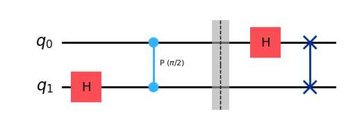
np.allclose(Operator(qft2), F_4)

True

Example: QFT on 3 qubits

qft3 = QuantumCircuit(3)
qft3.h(2)
qft3.cp(np.pi/2, 2, 1) 
qft3.cp(np.pi/4, 2, 0)
qft3.barrier()
qft3.h(1)
qft3.cp(np.pi/2, 1, 0)
qft3.barrier()
qft3.h(0)
qft3.swap(0, 2) # little endian ...
qft3.draw(output="mpl", style="iqp")

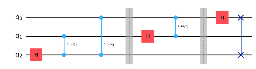
np.allclose(Operator(qft3), mk_F(8))

True

Arbitrary qubits

1. You can use the recurrence relation to write the circuit for arbitrary quibits.

2. See https://qiskit.org/textbook/ch-algorithms/quantum-fourier-transform.html

def qft(circuit, n):
    def go(circuit, n):
        if n == 0:
            return circuit
        else:
            n -= 1
            # Apply H
            circuit.h(n)
            # Apply CR
            for qubit in range(n):
                circuit.cp(np.pi/2**(n-qubit), qubit, n)
            # Recurrence relation
            return go(circuit, n)
    circuit = go(circuit, n) 

    # Take care of little endian
    for qubit in range(n//2):
        circuit.swap(qubit, n-qubit-1)
    return circuit

qft3_ = QuantumCircuit(3)
qft3_ = qft(qft3_, 3)
qft3_.draw(output="mpl", style="iqp")

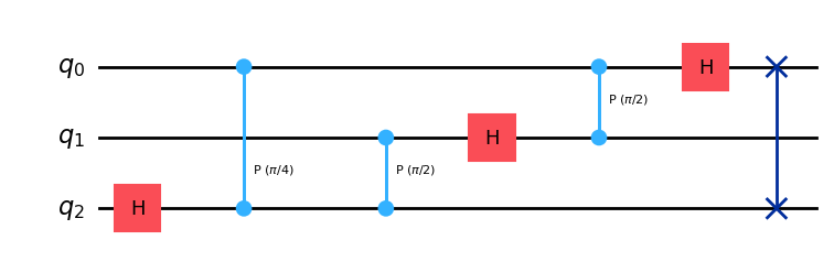
np.allclose(Operator(qft3), Operator(qft3_))

True

How many gates?

Note that

\[ t + (t - 1) + \dots 1 = \frac{t(t - 1)}{2} \,. \]

Thus we require \(O(t^2)\) gates.

Summary

1. The QFT performs a change-of-basis that enables us to store information in the global phase.

2. Later, we will use the quantum phase estimation (QPE) algorithm to read this information out.