import random
import numpy as np
import matplotlib.pyplot as plt
from typing import *

from qiskit_aer import AerSimulator
import qiskit.quantum_info as qi
from qiskit.quantum_info import Statevector, Operator
from qiskit.visualization import plot_histogram
from qiskit import QuantumCircuit
sim = AerSimulator()

from util import zero, one, Pretty

QI: Mixed States and Density Matrices

In this notebook, we’ll introduce density matrices. Density matrices enable us to describe mixed states which are statical ensembles of quantum states. Mixed states can arise due to decoherence/noise or due to partial measurement.

1. Quantum Computation and Quantum Information: Chapter 2.4, Nielsen and Chuang

2. https://qiskit.org/textbook/ch-quantum-hardware/density-matrix.html

Mixed States

A collection

\[ \{ (p_1, |v_1\rangle), \dots, (p_n, |v_n\rangle) \} \]

where \(|v_i\rangle\) are quantum state vectors and \(\sum_{i=1}^n p_i = 1\) is a mixed state. We can interpret a mixed state as a classic probability distribution over quantum state vectors. Thus we can also call a mixed state an ensemble.

Examples

We’ll unpack the definition with a few examples.

Example 1

We’ll first look at a mixed state over a single qubit system to contrast an ensemble and superposition.

X1 = [zero, one]
ps1 = [0.5, 0.5]
ensemble1 = [(p, x) for p, x in zip(ps1, X1)]
ensemble1

[(0.5,
  Statevector([1.+0.j, 0.+0.j],
              dims=(2,))),
 (0.5,
  Statevector([0.+0.j, 1.+0.j],
              dims=(2,)))]

samples = random.choices(
    [str(x) for p, x in ensemble1],
    weights=[p for p, x in ensemble1],
    k=1000
)
plt.hist(samples); plt.title("Ensemble 1")

Text(0.5, 1.0, 'Ensemble 1')

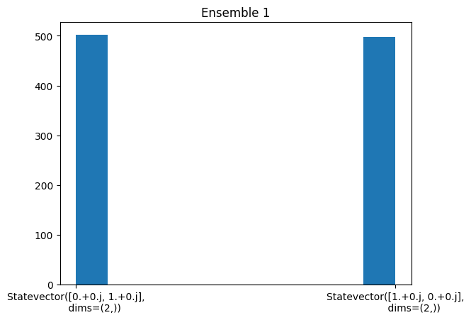
1. The mixed state given by ensemble 1 is either \(|0\rangle\) or \(|1\rangle\) with 50% probability.

2. The mixed state is different from the state \(\frac{1}{\sqrt{2}}(|0\rangle + |1\rangle)\) that is an equal superposition of \(|0\rangle\) and \(|1\rangle\) with 100% probability.

3. Upon measurement, we still obtain that \(\frac{1}{\sqrt{2}}(|0\rangle + |1\rangle)\) gives either \(|0\rangle\) or \(|1\rangle\) with 50% probability.

Example 2

Our next example looks at a mixed state over a single qubit involving 3 components.

# Can overspecify
X2 = [zero, one, 1/np.sqrt(2)*zero + 1/np.sqrt(2)*one]
ps2 = [0.2, 0.5, 0.3]
ensemble2 = [(p, x) for p, x in zip(ps2, X2)]
ensemble2

[(0.2,
  Statevector([1.+0.j, 0.+0.j],
              dims=(2,))),
 (0.5,
  Statevector([0.+0.j, 1.+0.j],
              dims=(2,))),
 (0.3,
  Statevector([0.70710678+0.j, 0.70710678+0.j],
              dims=(2,)))]

samples = random.choices(
    [str(x) for p, x in ensemble2],
    weights=[p for p, x in ensemble2],
    k=1000
)
fig, axes = plt.subplots(1, 1); plt.hist(samples)
plt.setp(axes.get_xticklabels(), rotation=10, horizontalalignment='right');

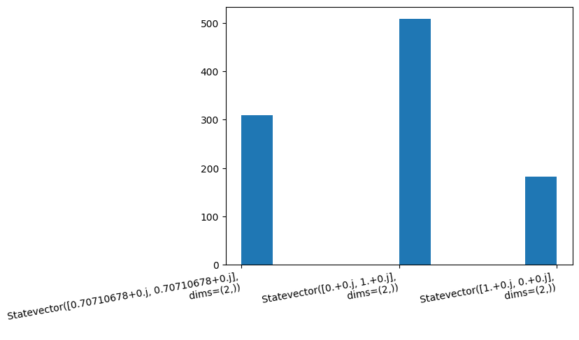
1. The mixed state given by ensemble 2 is either \(|0\rangle\) (30%), \(|1\rangle\) (50%), or \(\frac{1}{\sqrt{2}}(|0\rangle + |1\rangle)\) (20%).

2. Upon measurement, we obtain \(|0\rangle\) with probability 35% and \(|1\rangle\) with 65% probability.

Example 3

Our final example introduces one over a multi-qubit system.

# Can underspecify (missing one ^ zero)
X3 = [zero ^ zero, one ^ one, zero ^ one]
ps3 = [0.3, 0.2, 0.5]
ensemble3 = [(p, x) for p, x in zip(ps3, X3)]
ensemble3

[(0.3,
  Statevector([1.+0.j, 0.+0.j, 0.+0.j, 0.+0.j],
              dims=(2, 2))),
 (0.2,
  Statevector([0.+0.j, 0.+0.j, 0.+0.j, 1.+0.j],
              dims=(2, 2))),
 (0.5,
  Statevector([0.+0.j, 1.+0.j, 0.+0.j, 0.+0.j],
              dims=(2, 2)))]

samples = random.choices(
    [str(x) for p, x in ensemble3],
    weights=[p for p, x in ensemble3],
    k=1000
)
fig, axes = plt.subplots(1, 1); plt.hist(samples)
plt.setp(axes.get_xticklabels(), rotation=10, horizontalalignment='right');

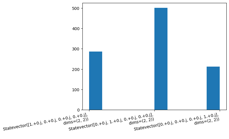
The mixed state given by ensemble 3 is either \(|00\rangle\) (30%), \(|11\rangle\) (20%), or \(|01\rangle\) (50%).

Mixed States vs. Pure States

The state of a quantum system given by an ordinary quantum state vector is called a pure state.

Motiviating Mixed States

Mixed states can arise due to decoherence/noise or due to partial measurement.

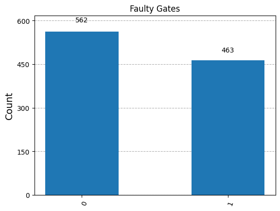
Situation 1: Decoherence/Noise

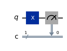
qc = QuantumCircuit(1, 1)
if np.random.rand() < 0.5:  # Suppose our hardware is faulty/noisy
    qc.x(0) # 50% of the time, we flip
else:
    qc.id(0) # 50% of the time, we don't do anything
qc.measure(0, 0)
qc.draw(output="mpl", style="iqp")

counts = {'0': 0, '1': 1}
for i in range(1024):
    qc = QuantumCircuit(1, 1)
    if np.random.rand() < 0.5:
        qc.x(0)
    else:
        qc.id(0)
    qc.measure(0, 0)
    state = sim.run(qc, shots=1).result()
    for k, v in state.get_counts().items():
        counts[k] += v
plot_histogram(counts, title='Faulty Gates')

Situation 2: Partial Measurement

Consider the following entangled state.

entangled = 1/np.sqrt(2)*(zero ^ zero) + 1/np.sqrt(2)*(one ^ one)
entangled.draw("latex")

\[\frac{\sqrt{2}}{2} |00\rangle+\frac{\sqrt{2}}{2} |11\rangle\]

Question

What can we say about the state of qubit 0 if we only measure qubit 1?

Answer

Let’s reason through this by running an experiment.

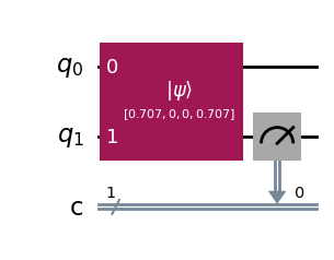
# Step 1: Prepare a measurement circuit
qc = QuantumCircuit(2, 1)
qc.initialize(entangled)
qc.measure(1, 0)
qc.draw(output="mpl", style="iqp")

# Step 2: Perform the measurement
state = sim.run(qc, shots=1024).result()
plot_histogram(state.get_counts(), title='Qubit 1 Results')

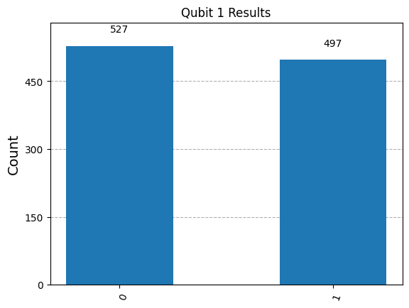
Analysis

1. After running the experiment, we see that qubit 1 is \(|0\rangle\) 50% of the time and \(|1\rangle\) 50% of the time.

2. Moreover, our 2-qubit system was entangled $\( \frac{1}{\sqrt{2}}|00\rangle + \frac{1}{\sqrt{2}}|11\rangle \,. \)$

3. If qubit 0 is \(|0\rangle\), then qubit 1 is \(|0\rangle\). Similarly, if qubit 0 is \(|1\rangle\), then qubit 0 is \(|0\rangle\).

4. However, measurement forces us to observe either \(|0\rangle\) or \(|1\rangle\) for qubit 1 with some probability, which by entanglement, forces this probability onto qubit \(0\).

5. We have recreated the mixed state given by ensemble 1!

Density Matrix

A density matrix provides an alternative characterization of mixed states and generalizes the notion of a quantum state vector.

Definition

Let \(\{ (p_1, |v_1\rangle), \dots, (p_n, |v_n\rangle) \}\) be an ensemble. A density matrix \(\rho\) is defined as

\[ \rho = \sum_{i=1}^n p_i |v_i\rangle \langle v_i| \]

where \(|v_i\rangle \langle v_i|\) is an outer product.

Aside: Outer Product

\[\begin{align*} |x\rangle \langle y| & = \begin{pmatrix} x_1 \\ \vdots \\ x_n \end{pmatrix} \begin{pmatrix} \overline{y_1} & \dots & \overline{y_m} \end{pmatrix} \tag{bra/ket} \\ & = \begin{pmatrix} x_1\overline{y_1} & \dots & x_1 \overline{y_m} \\ \vdots & \ddots & \vdots \\ x_n\overline{y_1} & \dots & x_n \overline{y_m} \\ \end{pmatrix} \tag{matrix multiplication} \end{align*}\]

Pretty(np.outer(np.array([1+1j, 1-1j, 2j]), np.array([1+1j, 1-1j])))

\[\begin{split}\begin{bmatrix} 2 i & 2 \\ 2 & - 2 i \\ -2 + 2 i & 2 + 2 i \\ \end{bmatrix} \end{split}\]

def ensembleToDensmat(ensemble: list[Tuple[float, Statevector]]) -> qi.DensityMatrix:
    return qi.DensityMatrix(sum([p * np.outer(x, x) for (p, x) in ensemble]))

Examples

ensemble1

[(0.5,
  Statevector([1.+0.j, 0.+0.j],
              dims=(2,))),
 (0.5,
  Statevector([0.+0.j, 1.+0.j],
              dims=(2,)))]

rho1 = ensembleToDensmat(ensemble1)
rho1.draw("latex")

\[\begin{split}\begin{bmatrix} \frac{1}{2} & 0 \\ 0 & \frac{1}{2} \\ \end{bmatrix} \end{split}\]

X15 = [1/np.sqrt(2) * zero + 1/np.sqrt(2)*one]
ps15 = [1.0]
ensemble15 = [(p, x) for p, x in zip(ps15, X15)]
rho15 = ensembleToDensmat(ensemble15)
rho15.draw("latex")

\[\begin{split}\begin{bmatrix} \frac{1}{2} & \frac{1}{2} \\ \frac{1}{2} & \frac{1}{2} \\ \end{bmatrix} \end{split}\]

ensemble2

[(0.2,
  Statevector([1.+0.j, 0.+0.j],
              dims=(2,))),
 (0.5,
  Statevector([0.+0.j, 1.+0.j],
              dims=(2,))),
 (0.3,
  Statevector([0.70710678+0.j, 0.70710678+0.j],
              dims=(2,)))]

rho2 = ensembleToDensmat(ensemble2)
Pretty(rho2)

\[\begin{split}\begin{bmatrix} \frac{7}{20} & \frac{3}{20} \\ \frac{3}{20} & \frac{13}{20} \\ \end{bmatrix} \end{split}\]

ensemble3

[(0.3,
  Statevector([1.+0.j, 0.+0.j, 0.+0.j, 0.+0.j],
              dims=(2, 2))),
 (0.2,
  Statevector([0.+0.j, 0.+0.j, 0.+0.j, 1.+0.j],
              dims=(2, 2))),
 (0.5,
  Statevector([0.+0.j, 1.+0.j, 0.+0.j, 0.+0.j],
              dims=(2, 2)))]

rho3 = ensembleToDensmat(ensemble3)
rho3.draw("latex")

\[\begin{split}\begin{bmatrix} \frac{3}{10} & 0 & 0 & 0 \\ 0 & \frac{1}{2} & 0 & 0 \\ 0 & 0 & 0 & 0 \\ 0 & 0 & 0 & \frac{1}{5} \\ \end{bmatrix} \end{split}\]

Observation 1: Sum of the diagonal is always 1

sum(np.diag(rho1)), sum(np.diag(rho2)), sum(np.diag(rho3))

(np.complex128(1+0j),
 np.complex128(0.9999999999999999+0j),
 np.complex128(1+0j))

Aside: Trace

Let

\[\begin{split} X = \begin{pmatrix} X_{11} & \dots & X_{1n} \\ \vdots & \ddots & \vdots \\ X_{n1} & \dots & X_{nn} \\ \end{pmatrix} \end{split}\]

be a square matrix.

Then

\[ Tr(X) = \sum_{i=1}^n X_{ii} \]

is the trace of a matrix.

np.trace(np.array([[1.0, 0.2], [0.3, 1.0]]))

np.float64(2.0)

np.trace(rho1), np.trace(rho2), np.trace(rho3)

(np.complex128(1+0j),
 np.complex128(0.9999999999999999+0j),
 np.complex128(1+0j))

Observation 1 more formally

Let \(\text{diag}\) obtain the diagonal of a matrix. Then

\[\begin{align*} Tr(\rho) & = Tr(\sum_{i=1}^n p_i \text{diag}(|v_i\rangle \langle v_i|)) \tag{definition} \\ & = \sum_{i=1}^n p_i Tr(|v_i\rangle \langle v_i|) \tag{trace properties} \\ & = \sum_{i=1}^n p_i (\sum_{j=1} v_{ij}\overline{v_{ij}}) \tag{outer product diagonal} \\ & = \sum_{i=1}^n p_i \tag{$\lVert v_i \rVert^2 = 1$} \\ & = 1 \tag{ensemble} \\ \end{align*}\]

Observation 2: Density matrix is Hermitian

Every density matrix is a Hermitian matrix, i.e.,

\[ X = X^\dagger \,. \]

print(np.allclose(rho1, np.conjugate(rho1).transpose()))
print(np.allclose(rho2, np.conjugate(rho2).transpose()))
print(np.allclose(rho3, np.conjugate(rho3).transpose()))

True
True
True

Observation 2 more formally

1. Recall

\[\begin{align*} |x\rangle \langle x| & = \begin{pmatrix} x_1\overline{x_1} & \dots & x_1 \overline{x_n} \\ \vdots & \ddots & \vdots \\ x_n\overline{x_1} & \dots & x_n \overline{x_n} \\ \end{pmatrix} \,. \end{align*}\]

2. Moreover, \(\overline{x_i \overline{x_j}} = \overline{x_i} x_j\).

3. Thus

\[\begin{align*} \begin{pmatrix} x_1\overline{x_1} & \dots & x_1 \overline{x_n} \\ \vdots & \ddots & \vdots \\ x_n\overline{x_1} & \dots & x_n \overline{x_n} \\ \end{pmatrix}^\dagger & = \begin{pmatrix} \overline{x_1}x_1 & \dots & \overline{x_1} x_n \\ \vdots & \ddots & \vdots \\ \overline{x_n}x_1 & \dots & \overline{x_n} x_n \\ \end{pmatrix}^T \\ & = \begin{pmatrix} x_1\overline{x_1} & \dots & x_1 \overline{x_n} \\ \vdots & \ddots & \vdots \\ x_n\overline{x_1} & \dots & x_n \overline{x_n} \\ \end{pmatrix} \end{align*}\]

Observation 3: Non-zero non-diagonal entries measures “quantumness”

# No superposition between |0> or |1>
print("Ensemble", ensemble1)
print("Purity", rho1.purity())
rho1.draw("latex")

Ensemble [(0.5, Statevector([1.+0.j, 0.+0.j],
            dims=(2,))), (0.5, Statevector([0.+0.j, 1.+0.j],
            dims=(2,)))]
Purity (0.5+0j)

\[\begin{split}\begin{bmatrix} \frac{1}{2} & 0 \\ 0 & \frac{1}{2} \\ \end{bmatrix} \end{split}\]

# Superposition between |0> or |1>
print("Ensemble", ensemble2)
print("Purity", rho2.purity())
rho2.draw("latex")

Ensemble [(0.2, Statevector([1.+0.j, 0.+0.j],
            dims=(2,))), (0.5, Statevector([0.+0.j, 1.+0.j],
            dims=(2,))), (0.3, Statevector([0.70710678+0.j, 0.70710678+0.j],
            dims=(2,)))]
Purity (0.5899999999999999+0j)

\[\begin{split}\begin{bmatrix} \frac{7}{20} & \frac{3}{20} \\ \frac{3}{20} & \frac{13}{20} \\ \end{bmatrix} \end{split}\]

Density Matrix Formulation of Quantum Computation

We reformulate quantum computation using density matrices. This includes

1. reformulating the quantum state representation,

2. unitary evolution, and

3. measurement.

Quantum State Representation

Every quantum state vector \(|v\rangle\) maps to the ensemble \(\{(1, |v\rangle)\}\)

v = 1/np.sqrt(2)*zero + 1/np.sqrt(2)*one
v.draw("latex")

\[\frac{\sqrt{2}}{2} |0\rangle+\frac{\sqrt{2}}{2} |1\rangle\]

qi.DensityMatrix(v).draw("latex")

\[\begin{split}\begin{bmatrix} \frac{1}{2} & \frac{1}{2} \\ \frac{1}{2} & \frac{1}{2} \\ \end{bmatrix} \end{split}\]

Unitary Evolution

The equivalent evolution of a density matrix \(\rho_{start} = |\psi\rangle \langle \psi|\) by \(U\) is given by

\[ \rho_{final} = U \rho_{start} U^\dagger \,. \]

Recall: Quantum state vector evolution

Given a quantum state vector \(|\psi\rangle\) and a unitary transformation \(U\), the result of applying \(U\) was \(U|\psi\rangle\).

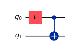
# Construct circuit
qc = QuantumCircuit(2)
qc.h(0)
qc.cx(0, 1)
qc.draw(output="mpl", style="iqp")

# Corresponding unitary transformation
U = Operator(qc)
U.draw("latex")

\[\begin{split}\begin{bmatrix} \frac{\sqrt{2}}{2} & \frac{\sqrt{2}}{2} & 0 & 0 \\ 0 & 0 & \frac{\sqrt{2}}{2} & - \frac{\sqrt{2}}{2} \\ 0 & 0 & \frac{\sqrt{2}}{2} & \frac{\sqrt{2}}{2} \\ \frac{\sqrt{2}}{2} & - \frac{\sqrt{2}}{2} & 0 & 0 \\ \end{bmatrix} \end{split}\]

print("Final state calculated with unitary evolution ...")
start = zero ^ zero
final = start.evolve(U)
final.draw("latex")

Final state calculated with unitary evolution ...

\[\frac{\sqrt{2}}{2} |00\rangle+\frac{\sqrt{2}}{2} |11\rangle\]

print("Final density matrix calculated with density matrix evolution ...")
qi.DensityMatrix(start).evolve(U).draw("latex")

Final density matrix calculated with density matrix evolution ...

\[\begin{split}\begin{bmatrix} \frac{1}{2} & 0 & 0 & \frac{1}{2} \\ 0 & 0 & 0 & 0 \\ 0 & 0 & 0 & 0 \\ \frac{1}{2} & 0 & 0 & \frac{1}{2} \\ \end{bmatrix} \end{split}\]

print("Do unitary evolution and density matrix evolution match?", np.allclose(qi.DensityMatrix(start).evolve(U), qi.DensityMatrix(final)))

Do unitary evolution and density matrix evolution match? True

Measurement

1. Let \(\{ \Pi_m \}_m\) be a complete set of measurement operators where \(m\) refers to the outcome so that it satisfies

\[ \sum_m \Pi_m^\dagger \Pi_m = I \,. \]

2. Then the probability of obtaining outcome \(m\) after measuring is

\[ p(m) = tr(\Pi_m^\dagger \Pi_m \rho) \,. \]

3. The state of the system after measurement is

\[ \frac{\Pi_m \rho \Pi_m^\dagger}{tr(\Pi_m^\dagger \Pi_m \rho)} \,. \]

def measure_outcome(rho: qi.DensityMatrix, M_m: np.ndarray) -> Tuple[float, qi.DensityMatrix]:
    # Probability of measuring m
    p_m = np.trace(np.conjugate(M_m.transpose()) @ M_m @ rho.data)

    # Resulting state after m
    rho_p = (M_m @ rho.data @ np.conjugate(M_m.transpose())) / p_m
    
    return p_m, rho_p

Example: Bell State

We’ll check that the reformulation of measurement matches on the Bell state. First, we recall the entangling circuit that created the Bell state.

qc.draw(output="mpl", style="iqp")

(zero ^ zero).evolve(qc).draw("latex")

\[\frac{\sqrt{2}}{2} |00\rangle+\frac{\sqrt{2}}{2} |11\rangle\]

rho = qi.DensityMatrix(qc)
rho.draw("latex")

\[\begin{split}\begin{bmatrix} \frac{1}{2} & 0 & 0 & \frac{1}{2} \\ 0 & 0 & 0 & 0 \\ 0 & 0 & 0 & 0 \\ \frac{1}{2} & 0 & 0 & \frac{1}{2} \\ \end{bmatrix} \end{split}\]

Recall that our measurement operators for partially measuring the first qubit (\(|q_0\rangle\)) were

1. \(\Pi_{*0} = |00\rangle\langle 00| + |10\rangle\langle 10|\) and

2. \(\Pi_{*1} = |01\rangle\langle 01| + |11\rangle\langle 11|\).

zz = zero ^ zero; zo = zero ^ one; oz = one ^ zero; oo = one ^ one
Pi0s = np.outer(zz, zz) + np.outer(oz, oz) # Pi0s only observes 1st qubit, and we get 0
Pi1s = np.outer(zo, zo) + np.outer(oo, oo) # Pi1s only observes 1st qubit, and we get 1
Pretty(Pi0s + Pi1s)

\[\begin{split}\begin{bmatrix} 1 & 0 & 0 & 0 \\ 0 & 1 & 0 & 0 \\ 0 & 0 & 1 & 0 \\ 0 & 0 & 0 & 1 \\ \end{bmatrix} \end{split}\]

We’ll check the result of measuring \(|q_0\rangle\) and obtaining \(0\).

p_0, rho_0 = measure_outcome(rho, Pi0s)
print("probability |0>", p_0)
print("resulting density matrix")
# Note that we can express measurement of partial states
Pretty(rho_0)

probability |0> (0.4999999999999999+0j)
resulting density matrix

\[\begin{split}\begin{bmatrix} 1 & 0 & 0 & 0 \\ 0 & 0 & 0 & 0 \\ 0 & 0 & 0 & 0 \\ 0 & 0 & 0 & 0 \\ \end{bmatrix} \end{split}\]

Similarly, we’ll check the result of measuring \(|q_0\rangle\) and obtaining \(1\).

p_1, rho_1 = measure_outcome(rho, Pi1s)
print("probability |1>", p_1)
print("resulting density matrix")
# Note that we can express measurement of partial states
Pretty(rho_1)

probability |1> (0.4999999999999999+0j)
resulting density matrix

\[\begin{split}\begin{bmatrix} 0 & 0 & 0 & 0 \\ 0 & 0 & 0 & 0 \\ 0 & 0 & 0 & 0 \\ 0 & 0 & 0 & 1 \\ \end{bmatrix} \end{split}\]

Summary

1. Introduced mixed states and density matrices, which are fundamental abstractions in QIS.

2. We Reformulated the unitary evolution of quantum states in terms of density matrices.