import matplotlib.pyplot as plt
import numpy as np
from typing import *

from qiskit import QuantumCircuit
from qiskit.quantum_info import Statevector, Operator
from qiskit_aer import AerSimulator
sim = AerSimulator()

from util import zero, one, qft

Shor’s Part 3/5: Modular Exponentiation

References

1. Introduction to Classical and Quantum Computing, Chapter 7.9.3

2. Qiskit notebook on Shor’s Algorithm

3. Introduction to Quantum Information Science: Lecture 19 by Scott Aaronson

4. Quantum Computation and Quantum Information: Chapter 5, Nielsen and Chuang

Quantum Oracle for Modular Multiplication

1. Suppose we have a unitary

\[ U_f |y \rangle = |ay \, (\text{mod} \, N) \rangle \]

so that \(U_f\) encodes modular multiplication by \(a\). This oracle will be useful for quantum order finding.

2. Question: why don’t we need an xor oracle?

Example

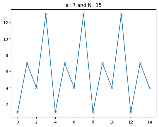
Consider

\[ f(x) = a^x \, (\text{mod} \, N) \]

where \(a = 7\) and \(N = 15\).

a = 7; N = 15
xs = [x for x in range(N)]
ys = [(a ** x) % N for x in xs]
plt.plot(xs, ys, marker='x'); plt.title("a=7 and N=15")

Text(0.5, 1.0, 'a=7 and N=15')

Quantum Oracle

1. Let \(y = y_4 y_3 y_2 y_1\) be the binary expansion of \(y\) in 4 bits where \(y_4\) is the most significant bit.

2. Our goal is to construct the unitary

\[ U_f |y \rangle = |0111 \cdot y \, (\text{mod} \, 1111) \rangle \]

where \(7 = 0111\) and \(15 = 1111\).

def amod15(a, power):
    # Adapted From: https://qiskit.org/textbook/ch-algorithms/shor.html
    if a not in [2,4,7,8,11,13]:
        raise ValueError("'a' must be 2,4,7,8,11 or 13")
    U = QuantumCircuit(4)        
    for iteration in range(power):
        if a in [2,13]:
            U.swap(2,3); U.swap(1,2); U.swap(0,1)
        if a in [7,8]:
            U.swap(0,1); U.swap(1,2); U.swap(2,3)
        if a in [4, 11]:
            U.swap(1,3); U.swap(0,2)
        if a in [7,11,13]:
            for q in range(4):
                U.x(q)
    U = U.to_gate(); U.name = "%i^%i mod 15" % (a, power); 
    return U

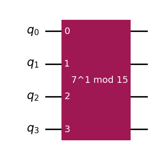
qc_amod15 = QuantumCircuit(4)
qc_amod15.append(amod15(7, 2**0), [0, 1, 2, 3])
U_f = Operator(qc_amod15)
qc_amod15.draw(output="mpl", style="iqp")

print((1 * 7) % 15) # Check that we get binary 7 (little endian)
(zero ^ zero ^ zero ^ one).evolve(U_f).draw("latex")

7

\[ |0111\rangle\]

print((3 * 7) % 15) # Check that we get binary 6 (little endian)
(zero ^ zero ^ one ^ one).evolve(U_f).draw("latex")

6

\[ |0110\rangle\]

Iterating Applications of \(U_f\)

1. Observe that if we iteratively apply \(U_f\) to itself

\[\begin{align*} U_f |0001 \rangle & = |a \, (\text{mod} \, N) \rangle \\ U_f^2 |0001 \rangle & = |a^2 \, (\text{mod} \, N) \rangle \\ \vdots & = \vdots \\ U_f^{s-1} |0001 \rangle & = |a^{s-1} \, (\text{mod} \, N) \rangle \\ U_f^{s} |0001 \rangle & = |a^s \, (\text{mod} \, N) \rangle \\ & = |0001 \rangle \,. \\ \end{align*}\]

2. Thus we can encode the original function as

\[ f(x) = U_f^x |0001\rangle \]

so that we can sequence \(U_f\) \(x\) times to simulate \(f(x)\).

# Starting vector  (reminder: little endian)
(zero ^ zero ^ zero ^ one).draw("latex")

\[ |0001\rangle\]

# U_f |0001>   (reminder: little endian)
(zero ^ zero ^ zero ^ one).evolve(U_f).draw("latex")

\[ |0111\rangle\]

U_f2 = U_f.compose(U_f)
# U_f^2 |0001>   (reminder: little endian)
(zero ^ zero ^ zero ^ one).evolve(U_f2).draw("latex")

\[ |0100\rangle\]

U_f3 = U_f.compose(U_f2)
# U_f^3 |0001>   (reminder: little endian)
(zero ^ zero ^ zero ^ one).evolve(U_f3).draw("latex")

\[ |1101\rangle\]

U_f4 = U_f.compose(U_f3)
# U_f^4 |0011> = |0001>   (reminder: little endian)
# Recall that the order was 4
(zero ^ zero ^ zero ^ one).evolve(U_f4).draw("latex")

\[ |0001\rangle\]

Aside: Eigenvectors and Eigenvalues

We say that \(x\) is an eigenvector and \(\lambda\) is an eigenvalue of a matrix \(A\) if

\[ Ax = \lambda x \,. \]

Eigenvectors and eigenvalues of \(U_f\)

1. \(|0001\rangle\) is an eigenvector of \(U_f\) with eigenvalue \(1\).

2. Are there other eigenvectors/eigenvalues of \(U_f\)?

3. Let

\[ |u\rangle = \frac{1}{\sqrt{s}} \sum_{k=0}^{s-1} U_f^k |1\rangle \]

be an equal superposition of the powers of \(U_f\). Then

\[\begin{align*} U_f |u\rangle & = U_f \left( \frac{1}{\sqrt{s}} \sum_{k=0}^{s-1} U_f^k |1\rangle \right) \tag{definition} \\ & = \left( \frac{1}{\sqrt{s}} \sum_{k=0}^{s-1} U_f^{k+1} |1\rangle \right) \tag{linearity} \\ & = \left( \frac{1}{\sqrt{s}} \sum_{k=0}^{s-1} U_f^{k} |1\rangle \right) \tag{$U_f^0 = U_f^s$} \\ & = |u\rangle \tag{definition} \end{align*}\]

(1/2.*((zero ^ zero ^ zero ^ one).evolve(U_f) +
(zero ^ zero ^ zero ^ one).evolve(U_f2) +
(zero ^ zero ^ zero ^ one).evolve(U_f3) +
(zero ^ zero ^ zero ^ one))).draw("latex")

\[\frac{1}{2} |0001\rangle+\frac{1}{2} |0100\rangle+\frac{1}{2} |0111\rangle+\frac{1}{2} |1101\rangle\]

# Checking eigenvector
(1/2.*((zero ^ zero ^ zero ^ one).evolve(U_f) +
(zero ^ zero ^ zero ^ one).evolve(U_f2) +
(zero ^ zero ^ zero ^ one).evolve(U_f3) +
(zero ^ zero ^ zero ^ one))).evolve(U_f).draw("latex")

\[\frac{1}{2} |0001\rangle+\frac{1}{2} |0100\rangle+\frac{1}{2} |0111\rangle+\frac{1}{2} |1101\rangle\]

More useful eigenvectors and eigenvalues of \(U_f\)?

1. It is a fact that unitary matrices have unit norm eigenvalues.

2. Consequently, we might wonder if it possible to have phases \(e^{2\pi i k}\) as eigenvalues.

3. Where might we get such eigenvalues?

4. Let

\[ |u_\ell \rangle = \frac{1}{\sqrt{s}} \sum_{k=0}^{s-1} e^{-\frac{2\pi ik\ell}{s}} U_f^k |1\rangle \]

be an equal superposition of the powers of \(U_f\) with phase shifts \(e^{-\frac{2\pi ik\ell}{s}}\) .

5. Then

\[ U_f |u_\ell\rangle = e^{\frac{2\pi i\ell}{s}}|u_\ell\rangle \]

which means we leak out information about the period \(s\) in the global phase.

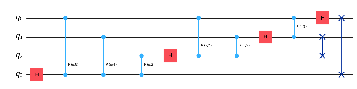
6. This is the change-of-basis given by the QFT.

qft4 = QuantumCircuit(4)
qft4 = qft(qft4, 4)
qft4.draw(output="mpl", style="iqp")

(zero ^ zero ^ zero ^ one).evolve(U_f).evolve(qft4).draw("latex")

\[\frac{1}{4} |0000\rangle+(-0.2309698831 + 0.0956708581 i) |0001\rangle+(0.1767766953 - 0.1767766953 i) |0010\rangle+(-0.0956708581 + 0.2309698831 i) |0011\rangle- \frac{i}{4} |0100\rangle+(0.0956708581 + 0.2309698831 i) |0101\rangle + \ldots +(0.0956708581 - 0.2309698831 i) |1011\rangle+\frac{i}{4} |1100\rangle+(-0.0956708581 - 0.2309698831 i) |1101\rangle+(0.1767766953 + 0.1767766953 i) |1110\rangle+(-0.2309698831 - 0.0956708581 i) |1111\rangle\]

Final fact: Sum of \(|u_\ell \rangle\)

One final observation is that

\[ |1\rangle = \frac{1}{\sqrt{s}} \sum_{\ell=0}^{s-1} |u_\ell \rangle \,. \]

Summary

We reviewed the quantum modular exponentiation algorithm.