import numpy as np
from typing import *

from qiskit import QuantumCircuit
from qiskit_aer import AerSimulator
from qiskit.quantum_info import Statevector, Operator
sim = AerSimulator()

from util import zero, one, PlotGateOpOnBloch, plot_bloch_vector

Foundations: Quantum Circuits for a Single Qubit System: Part 2

In this notebook, we will use the language of linear algebra to equivalently describe quantum circuits.

References

1. Introduction to Classical and Quantum Computing: Chapter 2

Quantum Gates and Unitary Matrices

A quantum gate \(G\) that acts on a single qubit system can be represented as a \(2 \times 2\) unitary matrix. That is, \(G \in \mathcal{U}(2)\) where \(\mathcal{U}(n)\) is the collection of unitary matrices in \(n\) dimensions. We’ll start with an example using the Hadamard gate.

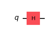
Example: Hadamard Gate

The unitary matrix

\[\begin{split} H = \frac{1}{\sqrt{2}} \begin{pmatrix} 1 & 1 \\ 1 & -1 \\ \end{pmatrix} \end{split}\]

encodes the Hadamard gate. We’ll characterize unitary matrix later.

qc_H = QuantumCircuit(1)
qc_H.h(0)
qc_H.draw(output="mpl", style="iqp")

# This produces the unitary matrix
H = Operator(qc_H)
H.draw("latex")

\[\begin{split}\begin{bmatrix} \frac{\sqrt{2}}{2} & \frac{\sqrt{2}}{2} \\ \frac{\sqrt{2}}{2} & - \frac{\sqrt{2}}{2} \\ \end{bmatrix} \end{split}\]

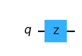
Example: Z Gate

The unitary matrix

\[\begin{split} Z = \frac{1}{\sqrt{2}} \begin{pmatrix} 1 & 0 \\ 0 & -1 \\ \end{pmatrix} \end{split}\]

encodes the \(Z\) gate.

qc_Z = QuantumCircuit(1)
qc_Z.z(0)
qc_Z.draw(output="mpl", style="iqp")

Z = Operator(qc_Z)
Z.draw("latex")

\[\begin{split}\begin{bmatrix} 1 & 0 \\ 0 & -1 \\ \end{bmatrix} \end{split}\]

Example: Phase Gate

We can also construct a phase gate that performs a rotation around the \(Z\) axis on the Bloch sphere by \(\lambda\) radians as in

\[\begin{split} P(\lambda) = \begin{pmatrix} 1 & 0 \\ 0 & e^{i\lambda} \end{pmatrix} \,. \end{split}\]

qc_p = QuantumCircuit(1)
qc_p.p(np.pi, 0)
qc_p.draw(output="mpl", style="iqp")

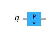
# A phase of 180 degrees is equivalent to a Z gate
def P(angle):
    qc_p = QuantumCircuit(1)
    qc_p.p(angle / 180 * np.pi, 0)
    return Operator(qc_p)
P(180).draw("latex")

\[\begin{split}\begin{bmatrix} 1 & 0 \\ 0 & -1 \\ \end{bmatrix} \end{split}\]

Gate Application is Matrix Multiplication

The application of a gate \(G\) to a qubit \(|q\rangle\) is notated

\[ G |q\rangle \]

and corresponds to the multiplication of the corresponding \(2 \times 2\) unitary matrix to the quantum state encoded by \(|q\rangle\).

Example

Below, we show by example that matrix multiplication and the evolution of a quantum state under a gate are equivalent.

print("Matrix multiplication", np.array(Operator(qc_H)) @ np.array(zero))
(zero.evolve(Operator(qc_H))).draw('latex')

Matrix multiplication [0.70710678+0.j 0.70710678+0.j]

\[\frac{\sqrt{2}}{2} |0\rangle+\frac{\sqrt{2}}{2} |1\rangle\]

print("Matrix multiplication", np.array(Operator(qc_H)) @ np.array(one))
(one.evolve(Operator(qc_H))).draw('latex')

Matrix multiplication [ 0.70710678+0.j -0.70710678+0.j]

\[\frac{\sqrt{2}}{2} |0\rangle- \frac{\sqrt{2}}{2} |1\rangle\]

Unitary Matrix Review

Unitary matrices have two properties that are important for quantum computing:

1. invertible and

2. norm preservation.

Invertibility and Reversibility

Every unitary matrix is invertible. As a reminder, this means that for any unitary matrix \(U\), there exists another unitary matrix \(U^{-1}\) such that

\[ U U^{-1} = U^{-1} U = I \]

where \(I\) is the identity matrix. This means that that quantum computations are reversible, since the application of a gate \(U\) can always be undone by another gate \(U^{-1}\).

# This demonstrates that H is its own inverse
(Operator(qc_H) @ Operator(qc_H)).draw("latex")

\[\begin{split}\begin{bmatrix} 1 & 0 \\ 0 & 1 \\ \end{bmatrix} \end{split}\]

Conjugate Transpose

For a unitary matrix, the inverse takes a special form: it is the conjugate transpose, i..e.,

\[ U^{-1} = U^\dagger \,. \]

(P(30) @ np.conj(P(30)).T).draw("latex")

\[\begin{split}\begin{bmatrix} 1 & 0 \\ 0 & 1 \\ \end{bmatrix} \end{split}\]

Norm Preservation and Quantum Circuits

Every unitary matrix preserves the norm of the input vector. In symbols,

\[ \lVert U x \rVert = \lVert x \rVert \,. \]

# This demonstrates that H preserves the norm
np.linalg.norm(zero), np.linalg.norm(np.array(Operator(qc_H)) @ np.array(zero))

(np.float64(1.0), np.float64(0.9999999999999999))

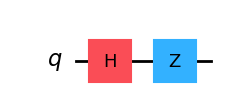
Sequencing Gates

The direct consequence of norm preservation is that applying a quantum gate to a single qubit produces an output that is also a qubit. This means that we can sequence the application of quantum gates to form a quantum computation as a quantum circuit. As a reminder, consider the circuit where we apply \(H\) followed by a \(Z\).

qc = QuantumCircuit(1)
qc.h(0)
qc.z(0)
qc.draw(output="mpl", style="iqp")

with PlotGateOpOnBloch() as ctx:
    plot_bloch_vector(zero, ax=ctx.ax1, title="Before H-Z")
    plot_bloch_vector(zero.evolve(Operator(qc)), ax=ctx.ax2, title="After H-Z")

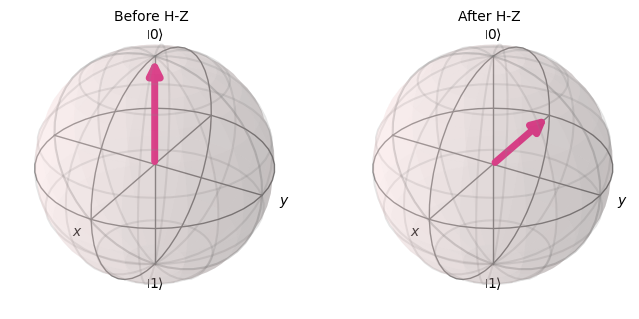
We can write the quantum circuit above using matrix multiplication as in

\[\begin{align*} |q_\text{output}\rangle & = ZH|0\rangle \tag{definition of circuit} \\ & = ZH \begin{pmatrix} 1 \\ 0 \end{pmatrix} \tag{substitute $|0\rangle$} \\ & = Z \frac{1}{\sqrt{2}} \begin{pmatrix} 1 & 1 \\ 1 & -1 \\ \end{pmatrix} \begin{pmatrix} 1 \\ 0 \end{pmatrix} \tag{substitute $H$} \\ & = Z \frac{1}{\sqrt{2}}(|0\rangle + |1\rangle) \tag{matrix multiplication} \\ & = \begin{pmatrix} 1 & 0 \\ 0 & -1 \end{pmatrix} \frac{1}{\sqrt{2}}(|0\rangle + |1\rangle) \tag{substitue $Z$} \\ & = \frac{1}{\sqrt{2}}(|0\rangle - |1\rangle) \tag{matrix multiplication} \,. \\ \end{align*}\]

Norm preservation ensures that

1. \(\lVert H|0\rangle \rVert = \lVert |0\rangle \rVert\) and

2. \(\lVert Z(H|0\rangle) \rVert = \lVert H|0\rangle \rVert\).

Since \(\lVert |0\rangle \rVert = 1\), we have that \(\lVert Z(H|0\rangle) \rVert = 1\) as well, so we have a valid quantum state.

# Initial
zero.draw("latex")

\[ |0\rangle\]

# Apply H
q1 = zero.evolve(H)
q1.draw("latex")

\[\frac{\sqrt{2}}{2} |0\rangle+\frac{\sqrt{2}}{2} |1\rangle\]

# Apply Z
q_after = q1.evolve(Z)
q_after.draw("latex")

\[\frac{\sqrt{2}}{2} |0\rangle- \frac{\sqrt{2}}{2} |1\rangle\]

Aisde: Order of H and Z

It may seem odd that the circuit is read left-to-right but the application of matrix multiplication was from right-to-left. However, forgetting quantum computation for a moment and considering in ordinary programming how we might apply \(H\) to an input, and then \(Z\), we’ll recognize that the order should be right-to-left.

def Z(x):
    return 2 * x

def H(x):
    return x + 1

print("Incorrect order for applying H, then Z:", H(Z(1)))
print("Correct order for apply H, then Z, is right-to-left:", Z(H(1)))

Incorrect order for applying H, then Z: 3
Correct order for apply H, then Z, is right-to-left: 4

Sequencing Gates corresponds to Matrix Multiplication

Alternatively, we can simplify the sequence of gate applications to a single “gate” by multiplying all the gates together. For example,

\[\begin{align*} ZH & = \begin{pmatrix} 1 & 0 \\ 0 & -1 \end{pmatrix}\frac{1}{\sqrt{2}} \begin{pmatrix} 1 & 1 \\ 1 & -1 \\ \end{pmatrix} \\ & = \frac{1}{\sqrt{2}} \begin{pmatrix} 1 & 1 \\ -1 & 1 \end{pmatrix} \,. \end{align*}\]

The quantum state can then be calculated as

\[\begin{align*} |q_\text{output}\rangle & = ZH|0\rangle \tag{definition of circuit} \\ & = ZH \begin{pmatrix} 1 \\ 0 \end{pmatrix} \tag{substitute $|0\rangle$} \\ & = \frac{1}{\sqrt{2}} \begin{pmatrix} 1 & 1 \\ -1 & 1 \end{pmatrix} \begin{pmatrix} 1 \\ 0 \end{pmatrix} \tag{substitute $ZH$} \\ & = \frac{1}{\sqrt{2}}(|0\rangle - |1\rangle) \tag{matrix multiplication} \end{align*}\]

H = Operator(qc_H)
Z = Operator(qc_Z)

ZH = Z @ H
ZH.draw("latex")

\[\begin{split}\begin{bmatrix} \frac{\sqrt{2}}{2} & \frac{\sqrt{2}}{2} \\ - \frac{\sqrt{2}}{2} & \frac{\sqrt{2}}{2} \\ \end{bmatrix} \end{split}\]

# Apply ZH
zero.evolve(Z @ H).draw("latex")

\[\frac{\sqrt{2}}{2} |0\rangle- \frac{\sqrt{2}}{2} |1\rangle\]

Reversibility and Sequencing

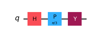
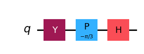
As we might guess, we can reverse the computation a sequence of gates performs by applying the inverse of each gate in reverse order.

qc = QuantumCircuit(1)
qc.h(0)
qc.p(np.pi / 3, 0)
qc.y(0)
qc.draw(output="mpl", style="iqp")

qc_rev = QuantumCircuit(1)
qc_rev.y(0)               # Y is it's own inverse
qc_rev.p(-np.pi / 3, 0)   # Rotate the other direction
qc_rev.h(0)               # H is it's own inverse
qc_rev.draw(output="mpl", style="iqp")

(Operator(qc) @ Operator(qc_rev)).draw("latex")

\[\begin{split}\begin{bmatrix} 1 & 0 \\ 0 & 1 \\ \end{bmatrix} \end{split}\]

Gate-Based Quantum Computing

1. In classical computation, we could encode an arbitrary truth table with circuits formed from a preselected set of gates (nand gates).

2. Similarly in gate-based quantum computing, we would try to encode an arbitrary transformation on a quantum state with quantum circuits from a preselected set of gates. In order to do this, we will need a universal gate set.

Summary

1. We reviewed the connection between \(2 \times 2\) unitary matrices and gates that act on a single qubit system.

2. We saw that every quantum computation was reversible.

3. The preservation of norm ensures that we can sequence the application of quantum gates to form a quantum circuit.