import numpy as np
import matplotlib.pyplot as plt

Appendix: Complex Numbers

We’ll review complex numbers (written \(\mathbb{C}\)). Complex numbers are integral to defining quantum states and quantum computations.

Definition of a Complex Number

A complex number \(z \in \mathbb{C}\) is a pair of real numbers \((a, b)\) typically written

\[ z = a + bj \,. \]

1. The number \(a\) is called the real component.

2. The number \(b\) is called the imaginary component. The letter \(j\) (or \(i\) is notation of imaginary).

An imaginary number is defined to be

\[ j = \sqrt{-1} \,. \]

You will more traditionally in mathematics see the notation

\[ i = \sqrt{-1} \,. \]

Examples

Some examples of complex numbers using numpy.

z1 = 1 + 2j
z1, z1.real, z1.imag

((1+2j), 1.0, 2.0)

z2 = .3 - .2j
z2, z2.real, z2.imag

((0.3-0.2j), 0.3, -0.2)

z3 = -2.4 + 3.2j
z3, z3.real, z3.imag

((-2.4+3.2j), -2.4, 3.2)

z4 = -1.4 - 1.2j
z4, z4.real, z4.imag

((-1.4-1.2j), -1.4, -1.2)

z5 = 1 + 0j  # Non-imaginary
z5, z5.real, z5.imag

((1+0j), 1.0, 0.0)

z6 = 0 + 1j  # Fully-imaginary
z6, z6.real, z6.imag

(1j, 0.0, 1.0)

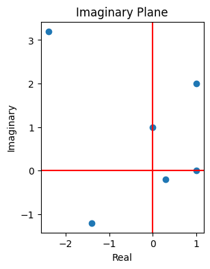
Imaginary Plane

A complex number can be represented as a point in the complex plane.

fig = plt.figure(figsize=(4, 4)); ax = fig.add_subplot()
ax.set_aspect(1.0/ax.get_data_ratio(), adjustable='box')

# Complex Numbers
zs = [z1, z2, z3, z4, z5, z6]
plt.plot([z.real for z in zs], [z.imag for z in zs], marker='o', linestyle='none')

# Plot meta-data
plt.axhline(y=0.0, color='r', linestyle='-'); plt.axvline(x=0.0, color='r', linestyle='-')
plt.xlabel('Real'); plt.ylabel('Imaginary'); plt.title('Imaginary Plane')

Text(0.5, 1.0, 'Imaginary Plane')

Operations on Complex Numbers

We’ll review operations on complex numbers, including arithmetic, the magnitude of a complex number, and complex conjugation.

Arithmetic on complex numbers

We can perform operations on complex numbers:

1. Addition: \((a + bj) + (c + dj) = (a + c) + (b + d)j\).

2. Negation: \(-(a + bj) = (-a) + (-b)j\).

3. Multiplication: \((a + bj) \cdot (c + dj) = (ac - bd) + (ad + bc)j\).

4. Inverse: \(1/(a + bj) = a/(a^2 + b^2) + (-b/(a^2 + b^2))j\).

z1 = (1 + 2j)
z2 = (.3 - .2j)
z1 + z2, z1.real + z2.real + (z1.imag + z2.imag)*1j

((1.3+1.8j), (1.3+1.8j))

z1 = (1 + 2j)
-z1, -z1.real + (-z1.imag)*1j

((-1-2j), (-1-2j))

# Subtraction is addition of negation
z1 = (1 + 2j)
z2 = (.3 - .2j)
z1 - z2, z1.real - z2.real + (z1.imag - z2.imag)*1j

((0.7+2.2j), (0.7+2.2j))

z3 = -2.4 + 3.2j
z4 = -1.4 - 1.2j
z3 * z4

(7.199999999999999-1.5999999999999996j)

z2 = (.3 - .2j)
1 / z2

(2.3076923076923075+1.5384615384615385j)

Magnitude

The magnitude of a complex number is given by

\[ |a + bj| = \sqrt{a^2 + b^2} \,. \]

z1 = (1 + 2j)
np.abs(z1), np.sqrt(z1.real**2 + z1.imag**2)

(np.float64(2.23606797749979), np.float64(2.23606797749979))

z2 = (.3 - .2j)
np.abs(z2), np.sqrt(z2.real**2 + z2.imag**2)

(np.float64(0.3605551275463989), np.float64(0.36055512754639896))

Complex Conjugation

The complex conjugate of a complex number is given by

\[ \overline{a + bj} = a - bj\,. \]

z1 = (1 + 2j)
np.conjugate(z1)

np.complex128(1-2j)

z2 = (.3 - .2j)
np.conjugate(z2)

np.complex128(0.3+0.2j)

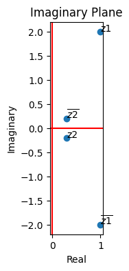
Geometric Intuition

1. Every operation on a complex number can be visualized in the complex plane.

2. For example, the complex conjugate of a number is a reflection over the real axis in the complex plane. Exercise: what is the geometric operation corresponding to negation?

fig = plt.figure(figsize=(4, 4)); ax = fig.add_subplot()
ax.set_aspect(1.0/ax.get_data_ratio(), adjustable='box')

# Complex Numbers
zs = [z1, np.conjugate(z1), z2, np.conjugate(z2)]; txt = ["z1", r"$\overline{z1}$", r"z2", r"$\overline{z2}$"]
plt.scatter([z.real for z in zs], [z.imag for z in zs])
for i, t in enumerate(txt):
    plt.annotate(t, (zs[i].real, zs[i].imag))

# Plot meta-data
plt.axhline(y=0.0, color='r', linestyle='-'); plt.axvline(x=0.0, color='r', linestyle='-')
plt.xlabel('Real'); plt.ylabel('Imaginary'); plt.title('Imaginary Plane');

Pairs of Complex Numbers

We will now introduce pairs of complex numbers \(\mathbb{C}^2\). We will write a pair of complex numbers using the notation

\[\begin{split} \begin{pmatrix} a \\ b \\ \end{pmatrix} \in \mathbb{C}^2 \end{split}\]

where \(a, b \in \mathbb{C}\) are complex numbers. We will see later that this is a vector space.

p1 = np.array([z1, z2])
z1, z2, p1

((1+2j), (0.3-0.2j), array([1. +2.j , 0.3-0.2j]))

p2 = np.array([z3, z4])
z3, z4, p2

((-2.4+3.2j), (-1.4-1.2j), array([-2.4+3.2j, -1.4-1.2j]))

Arithmetic on Complex Pairs

We can perform operations on pairs of complex number:

1. Addition:

\[\begin{split} \begin{pmatrix} a \\ b \end{pmatrix} + \begin{pmatrix} c \\ d \end{pmatrix} = \begin{pmatrix} a + c \\ b + d \end{pmatrix} \end{split}\]

2. Multiplication:

\[\begin{split} r\begin{pmatrix} a \\ b \end{pmatrix} = \begin{pmatrix} ra \\ rb \end{pmatrix} \end{split}\]

where \(r \in \mathbb{C}\).

p1, p2, p1 + p2

(array([1. +2.j , 0.3-0.2j]),
 array([-2.4+3.2j, -1.4-1.2j]),
 array([-1.4+5.2j, -1.1-1.4j]))

p1, -1 * p1

(array([1. +2.j , 0.3-0.2j]), array([-1. -2.j , -0.3+0.2j]))